Multivariate Linear Regression

1
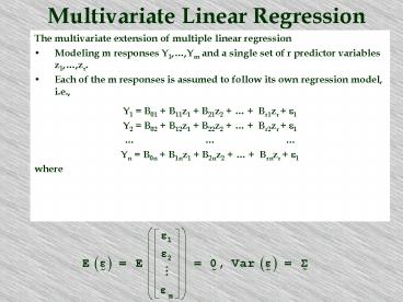
Multivariate Linear Regression

• The multivariate extension of multiple linear
  regression
• Modeling m responses Y1,,Ym and a single set of
  r predictor variables z1,,zr.
• Each of the m responses is assumed to follow its
  own regression model, i.e.,
• Y1 B01 B11z1 B21z2 Br1zr e1
• Y2 B02 B12z1 B22z2 Br2zr e1
• Yn B0n B1nz1 B2nz2 Brnzr e1
• where

n
2
Conceptually, we can let zj0, zj1, ,
zjr denote the values of the predictor
variables for the jth trial and
be the responses and errors for the jth trial.
Thus we have an n x (r 1) design matrix
3
If we now set
4
The multivariate linear regression model is
with
and

For example
5

The ordinary least squares estimates b are found
in a manner analogous to the univariate case we
begin by taking

collecting the univariate least squares
estimates yields
Now for any choice of parameters
the resulting matrix of errors is
6
The resulting Error Sums of Squares and
Crossproducts is

We can show that the selection b(i) b(i)
minimizes the ith diagonal sum of squares


generalized variance
i.e.,
are both minimized.
7
so we have matrices of predicted values
and we have a resulting matrices of residuals
Note that the orthogonality conditions which
hold in the univariate case are also true in the
multivariate case
8
which means the residuals are perpendicular to
the columns of the design matrix
and to the predicted values
Furthermore, because
we have
predicted sums of squares and crossproducts
residual (error) sums of squares and crossproducts
total sums of squares and crossproducts
9
Example suppose we had the following six
sample observations on two independent variables
(palatability and texture) and two dependent
variables (purchase intent and overall quality)
How is the multivariate linear regression model
formulated?
10
We wish to estimate Y1 B01 B11z1
B21z2 and Y2 B02 B12z1
B22z2 jointly. The design matrix is
11
so
and
12
and
so
13
and
so
14
so
This gives us estimated values matrix
15
and residuals matrix
Note that each column sums to zero!
16
Inference in Multivariate Regression
The least squares estimators b b(1) b(2)
?b(m) of the multivariate regression model
have the following properties - -
- if the model is of full rank, i.e., rank(Z)
r 1 lt n. Note that e and b are also
uncorrelated.







17
This means that, for any observation z0

is an unbiased estimator, i.e.,
We can also determine from these properties that
the estimation errors
have covariances
k
k
k
k
18
Furthermore

i.e., the forecasted vector Y0 associated with
the values of the predictor variables z0 is an
unbiased estimator of Y0. The forecast errors
have covariance



19
Thus, for the multivariate regression model with
full rank (Z) r 1, n ? r 1 m, and
normally distributed errors e,


is the maximum likelihood estimator of b and

where the elements of S are

20
Test for Ho b(2) 0
Define the Error Sum of Squares and
Crossproducts as E nS and the Hypothesis or
Extra Sum of Squares and Crossproducts as H
n(S1 - S) then we can define Wilks lambda as






where h1 ? h2 ? ? ? hs are the ordered
eigienvalues of HE-1 where s min(p, r - q).

21
There are other similar tests (as we have seen
in our discussion of MANOVA)
Pillais Trace Hotelling-Lawley Trace Roys
Greatest Root
Each of these statistics is an alternative to
Wilks lambda and perform in a very similar
manner (particularly for large sample sizes).
22
Example Regressing palatability and texture
onto purchase intent and overall quality
to test the hypotheses that i) palatability has
no joint relationship with purchase intent and
overall quality and ii) texture has no joint
relationship with purchase intent and overall
quality.
23
We first test the hypothesis that palatability
has no joint relationship with purchase intent
and overall quality, i.e., H0b(1) 0 The
test of this hypothesis is given by the ratio of
generalized variances as given by Wilks lambda
statistic

24
The error sum of squares and crossproducts
matrix is
and the hypothesis sum of squares and
crossproducts matrix for this null hypothesis is
25
so the calculated value of the Wilks lambda
statistic is
26
The transformation to a Chi-square distributed
statistic (which is actually valid only when n
r and n m are both large) is
at a 0.01 and m(r - q) 1 degrees of freedom,
the critical value is 9.210351. Not enough
evidence to reject H0 b(1) 0
27
We next test the hypothesis that texture has no
joint relationship with purchase intent and
overall quality, i.e., H0b(2) 0

The Chi-square transformation yields

Again, not enough evidence to reject H0 b(2) 0
28
We can also build confidence intervals for the
predicted mean value of Y0 associated with z0 -
if the model


has normal errors, then
and
independent
so
29
Thus the 100(1 a) confidence interval for the
predicted mean value of Y0 associated with z0
(bz0) is given by




and the 100(1 a) simultaneous confidence
intervals for the mean value of Yi associated
with z0 (z0 b(i) ) are




i 1,,m
30
Finally, we can build prediction intervals for
the predicted value of Y0 associated with z0
here the prediction error


has normal errors, then
and
independent
so
31
the prediction intervals the 100(1 a)
prediction interval associated with z0 is given by

and the 100(1 a) simultaneous prediction
intervals with z0 are

i 1,,m