CH3 : Linear methods for regression

1
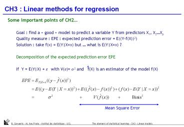
CH3 Linear methods for regression

• Some important points of CH2
• Goal find a  good  model to predict a
  variable Y from predictors X1, X2Xp
• Quality measure EPE expected prediction error
  E((Y-f(X))2)
• Solution take f(x) E(YXx) but what is
  E(YXx) ?
• Decomposition of the expected prediction error
  EPE
• If Y E(YX) e with V(e) s2 and f(X) is
  an estimator of the model f(X)

Mean Square Error
2
Linear regression models

• Linear regression models suppose that E(YX) is
  linear
• Linear models are old tools but
• Still very useful
• Simple
• Allow an easy interpretation of regressors
  effects
• Very wide since Xis can be any function of other
  variables (quantitative or qualitative)
• Useful to understand because most other methods
  are generalisations of them.

3
Least square estimation methods

• Least square is the most popular method to
  estimate linear models
• Least square criteria
• Solution of the minimisation problem
• Predicted values
• The predictions are the orthogonal projections of
  y in the subspace of Rn defined by the columns of
  the X matrix. H is the projection matrix.
• The method can be generalised to multiple Ys
• If the Yis are not correlated, the multivariate
  solution is identical than doing k classical
  regressions

4
Properties of least squares estimators

• If Yi are independent, X fixed and V(Yi)s2
  constant
• Then
• If, in addition, Yf(Xi)e with e N(0, s2 )
• Then
• and
• T tests can be built to test the nullity of one
  parameter
• F tests can be built to test the nullity of a
  vector of parameters (or linear combinations of
  them)
• Confidence intervals can be built for one of for
  a vector of parameters.
• Gauss-Markov theorem (does not need normality
  assumption)
• The least square estimates of the parameters b
  have the smallest variance among all linear
  UNBIASED estimators.
• But
• LS estimators do not have the small mean
  square error if one accepts biased estimators
  (e.g. ridge regression).
• and since all model are wrong, LSE will
  always be biased

5
Multiple regression from univariate regression

• Multiple regression parameters can be estimated
  from a sequence of simple univariate regressions
  of the type Y bz e
• If columns of X are orthogonal, the parameters
  estimates are simply simple regressions of Y on
  the columns of X
• The algorithm of successive orthogonalisation
  allows to obtain the estimator of bi in a
  multiple regression as the estimator of the
  parameter of a simple regression of Y on the
  residual Zi of the regression of Xi on the other
  columns of X. Zi is the part of Xi which is
  orthogonal to the space of the other columns of X
  and is obtained by a sequence of successive
  orthogonalisations.
• The Gram-Schmidt procedure is a numerical
  strategy based on the previous algorithm to
  compute LS estimates.
• These developments help to have a geometrical
  view of LS but will also be the basis of other
  algorithms (NIPALS for PCA, PLS)

6
Other methods to estimate linear models

• Two reasons why we are not happy with least
  squares
• Prediction accuracy LES often provide
  predictions with low biais but high variance.
• Intepretation when the number of regressors is
  to high, the model is difficult to interpret.
  One seek to find a smaller set of regressors with
  higher effects
• Proposed approaches
• Subset selection best subset, forward,
  backward, stepwise
• Shrinkage methods ridge regression and lasso
  method ( generalisation to a bayes view of them)
• Methods using derived input directions
  Principal component regression, partial least
  squares and canonical correlations

7
Proster cancer data example

• Variables
• response level of prostate-specific antigen
• Regressors 8 clinical measures useful for men
  receiving prostatectomy

8
Example results given

• For each method, the best compromise model is
  given
• The quality of the models are measured by tenfold
  cross-validation
• The data set is divided in ten parts, the model
  estimated by removing one by one each part and
  calculating the cross-validation prediction error
  on the m removed data.
• The test error is the mean of the CVks, the Std
  Error their standard deviation
• On the graph, the points are test errors and the
  intervals are at /- 1s of the test error
• The best model is the less complex model with a
  mean CV within /-1s of the best mean CV

9
Subset selection methods

• Idea retain only the subset of variables that
  gives the best fit. These are automatic methods
  without reflection on the nature of the
  regressors.
• Best subset regression
• all subset of k1,2,p regressors are tested and
  for each k the best model retained. Works for
  p
  criteria making a trade-off of bias and variance.
• Forward selection
• Starts with the intercept and add at each step
  the predictors that most improves the fit. The
  improvement is often measured with p-value of an
  F-test.
• Backward selection
• Starts with the full model and removes one by
  one the worst regressor. Stops when all
  regressors have a significant effect. Can only
  be used when p
• Stepwise selection
• Combines forward and backward to decide at each
  step which variable to remove and/or to add.

10
Shrinkage Methods Ridge Regression

• Shrink coefficients by imposing a penalty to
  their size

subject to
This is equivalent to
If inputs are orthogonal
Is a function of
11
Singular values decomposition (SVD)
Writing in terms of SVD
shrinked coordinates of y respect to U basis
Greater amount of shrinkage to basis vector
having smaller
Complexity parameter of the model
Effective degrees of freedom
12
Relationship with Principal Components
Writing in terms of SVD
Eigen decomposition
Normalized principal component
Principal components Normalized linear
combinations of the columns of X
Small values correspond to directions of
the column space of having small variance
Ridge regression assumes that response will tend
to vary the most in directions of higher variance
of the inputs and then it protects against high
variability of Y in directions of small
variability of X
13
Lasso regression
subject to
where

• If t is small enough some coefficients are 0,
  so it acts like a subset selection method
• If then

t is chosen to minimize de estimation of the
expected prediction error
14
Derived directions Principal Components
Regression
Use of linear combinations (PC)
as
regressors
Since the are orthogonal

• Ridge and PC regression operate via the principal
  components of the X matrix
• Ridge regression shrinks the regression
  coefficients of the principal components
  depending on the size of the corresponding
  eigenvalue.
• Principal component regression discard the
  smallest eigentvalues

15
Derived directions Partial Least Squares
Use a set of linear combinations of the inputs
also taking into account

• Standardize , set
  
• For
• .
• .
• .
  output
• . Orthogonalize with respect to
• .The coefficients on the original

16
Derived directions Partial Least Squares

• If M least squares
• Non linear function of y
• Look for directions with high variance and high
  correlation with y

PCR
PLS
Dominates, then behaves similar to Ridge and PCR
If X is orthogonal then
17
Multiple Outcome

• Least-squares individual least squares estimates
  to each output
• Selection and shrinkage methodsunivariate
  technique individually or simultaneously to all
  outcomes
• Ridge apply ridge regression to each column of
  , having different , or apply it to
  all columns with the same
• If correlation between the outputs
• Canonical correlation analysis (similar to PCA)
• Sequence of uncorrelated combinations on X ,
  and Y, such that
• are maximized
• Leading canonical responses are those linear
  combinations best predicted by the xs
• CCA solution is computed via SVD of the
  cross-covariance matrix
• Reduced-rank regression in terms of regression
  model. estimated by

Canonical vectors
18
Comparisons

• PLS, PCR and Ridge regression behave similarly.
• Ridge shrinks all directions but shrinks more low
  variance directions.
• PCR keeps higher variance Components and discard
  the rest.
• PLS shrink low-variance directions but tends to
  inflate some of the higher variance, causing
  slightly larger prediction error compared to
  ridge.
• Ridge is preferred for minimizing the prediction
  error and it shrinks smoothly
• If X is orthogonal, these methods apply simple
  transformations to the least square estimates. If
  X is not orthogonal, they converge to the least
  squares.