Monte Carlo Simulation of Canonical Distribution - PowerPoint PPT Presentation
Title:
Monte Carlo Simulation of Canonical Distribution
Description:
Pick a site at random and consider flipping it s = - s ... 2) compute the energy change if the spin is flipped E = E(new) E(old) ... – PowerPoint PPT presentation
Number of Views:247
Avg rating:3.0/5.0
Title: Monte Carlo Simulation of Canonical Distribution
1
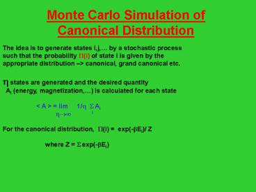
Monte Carlo Simulation of Canonical Distribution
The idea is to generate states i,j, by a
stochastic process such that the probability
?(i) of state i is given by the appropriate
distribution gt canonical, grand canonical
etc. ? states are generated and the desired
quantity Ai (energy, magnetization,) is
calculated for each state lt A
gt lim 1/? ? Ai
??? i For the canonical
distribution, ?(i) exp(-?Ei)/ Z
where Z ? exp(-?Ei)
2
How do we do this using a computer?
- Consider a system of N classical spins which can
be up or down. The total number of microstates is
M 2N - H -J ? si sj
- iltj
- We could generate configurations randomly and
calculate E(i) and weight its contribution by
exp(-?E(i)) - ltEgt ? E(i) exp(-?E(i)) / ? exp(-?E(i))
- Very inefficient since M 2N is exponentially
large. We can never generate all states if they
have equal probability and many configurations
make a small contribution - We want to use importance sampling!
3
Importance sampling
- ltAgt ? A(i)/?(i) exp(-?E(i)) ?(i)
- ? 1/?(i) exp(-?E(i)) ?(i)
- If we generate the microstates with probability
- ?(i) exp(-?E(i))/ ? exp(-?E(i))
- then ltAgt (1/n) ? A(i)
- How do we obtain ?(i) ?
4
Markov process
- Suppose the system is in state i. The next state
is selected with a transition probability P(j?i)
that does not depend on the previous history of
the system. - This process produces states with a unique
steady-state probability distribution (after a
transient) - The steady state probability ?(j) is an
eigenvector with eigenvalue 1 of the transition
matrix - ?(j) ? P(j?i) ?(i)
- i
5
Consider the following example A student changes
rooms at regular intervals and uses any of the
doors leaving the room with equal probability
What are the transition probabilities? What
fraction of the time will the student spend in
each room in a steady state?
Eg. if he is in room 2, then P(3?2) P(1?2)
1/2 Similarly, P(1?3) P(2?3) P(4?3) 1/3
6
Hence P(j?i) 0 1/2 1/3
0 1/2 0
1/3 0 1/2
1/2 0 1
0 0 1/3 0
- Eigenvalues are 1, -1/2, -1/4 ? 1/2 (11/12)1/2
- Eigenvector of largest eigenvalue is
( 1/4, 1/4, 3/8, 1/8) - Hence after a long time we reach a steady state
with - ?(1) 1/4 ?(2) 1/4 ?(3)3/8 ?(4)1/8
- Note ? ?(i) 1 (normalization)
- P(j?i) ?(i) P(i?j) ?(j) (detailed balance)
7
Ising Model
- Suppose system is in state i.
- Pick a site ? at random and consider flipping it
s? - s?. - The final state can be the same (i) or different
(j). After n steps - ?(f) lim P(f?i) ? P(f?in-1)
P(in-1?in-2) P(i1?i) - n??
- approaches a limiting distribution independent of
the initial state i. - We require ?(f) to be normalized and satisfy
- ?(m)/?(j) exp-?(E(m)-E(j)
for all pairs m,j - Normalization means ? P(j?m) 1
-
j - and P(j?m) ?(m) P(m?j) ?(j)
detailed balance - Hence ?(m) ? P(j?m) ?(m) ? P(m?j)
?(j) - j
j - ??(m) is a stationary probability distribution
8
Metropolis Algorithm
- 0) establish an initial microstate
- 1) pick site ? randomly
- 2) compute the energy change if the spin is
flipped ?E E(new) E(old) - 3) determine the value of A(i)
- 4) if ?E? 0, then flip it and proceed to 7
- 5) if ?Egt0, then compute we-??E
- 6) generate a random number r
- 7) if r? w accept the new state otherwise remain
in the old - 8) repeat steps 1) to 7)
- 9) Calculate ltAgt and ltA2gt-ltAgt2
9
Periodic boundary conditions
10
Specific heat and magnetic susceptibility
Cv ltE2gt-ltEgt2
kT2 ?
ltM2gt-ltMgt2
kT e.g. Ising Model Si ? 1 on a square
lattice of NL2 sites In the limit L?? , the
exact results are known
11
(No Transcript)
12
In the limit as L ?? the system undergoes a
phase transition The exact Tc
2.269185 The specific heat diverges
logarithmically
Cv lnT-Tc The susceptibility
diverges as
? T-Tc-? with ?7/4
13
Monte Carlo Simulation of the Ising Model
14
This is an example of an order- disorder
transition F E - TS energy(order) versus
entropy(disorder)
- In d1, the ground state at T0 has all spins
aligned parallel ????????????????????????????? - Low energy excitations correspond to domain walls
?????????????????????????????? - ?E 2J ?S k ln(N)
- ?F 2J- kT ln(N) lt 0
- The ordered phase is unstable at finite Tgt0
towards the formation of defects (domain walls)
15
d2
On the square lattice, the ground state has all
spins aligned parallel
??????? ??????? ???????
Low energy excitations consist of compact
clusters(domains) of
overturned spins
??????? ??????? r8 ???????
?E 2J r , ?S k ln(3r) r is the
perimeter of the cluster
Hence ?F ? 2J- kT ln(3) r rgtgt1
At low T, ?F is positive but vanishes at a finite
T


