2D Non-linear version of Mixed Spectral Finite Difference model. - PowerPoint PPT Presentation
Title:
2D Non-linear version of Mixed Spectral Finite Difference model.
Description:
2D Non-linear version of Mixed Spectral Finite Difference model. Xiao Yu a, Wensong Weng b, Peter A Taylor b, Dong Liang a a Department of Mathematics and Statistics ... – PowerPoint PPT presentation
Number of Views:25
Avg rating:3.0/5.0
Title: 2D Non-linear version of Mixed Spectral Finite Difference model.
1
2D Non-linear version of Mixed Spectral Finite
Difference model. Xiao Yu a, Wensong Weng b,
Peter A Taylor b, Dong Liang a a Department of
Mathematics and Statistics, York University, 4700
Keele Street, Toronto, Ontario, Canada M3J 1P3 b
Department of Earth and Space Science and
Engineering, York University, Toronto, Ontario,
Canada M3J 1P3
In the Bolund comparison, our group used a 2D
non-linear version of the mixed spectral finite
difference method (NLMSFD) for flow over
topography with E-?z closure. A linearized
version (MSFD) from Beljaars et al (1987) applies
a Fourier transform in horizontal coordinates and
uses finite differences in the vertical
coordinate. The non-linear extension (NLMSFD) was
then developed by Xu and Taylor (1992) with
non-linear terms treated as additional source
terms (in R below), L(
f )R( f(n-1) ) f (n)
?f (1-?)f(n-1) . This model was
limited to a maximum slope of 0.3 due to
stability of the iteration scheme, but it still
can be improved by choosing a smaller relaxation
factor. The 3D version of NLMSFD still had
problems with Bolund terrain at this moment,
therefore a 2D NLMSFD is presented here for
calculations on Line A and Line B. Roughness
changes are treated separately.
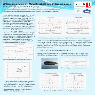
Horizontal x component velocity profiles in case
1 (wind from 270) and case 3 (wind from 239).
Due to limitations of the 2D model used, we are
only able to calculate those points lying on Line
B in case 1 and case 4, and points lying on Line
A in case 3. A roughness length of z00.015 m is
used for computing topographic effects. Wind
speed changes caused by roughness changes are
computed from the PBL roughness change flow model
of Weng et al. To rescale and combine results we
set, UU0(Z) (1 ?St(X, Z) )/(1
?St(-400 m, Z) )?Sr(X, Z) , where U0(Z) is the
upstream profile, ?St is the fractional speed-up
ratio for terrain from NLMSFD and ?Sr is
fractional speed-up ratio for roughness change
from the PBL model.
Fractional speed-up ratio in case 1. Adjusted to
give ?St(-400 m, Z) 0.
Line A
Surface smoothing is used to reduce the maximum
slope.
Line B
The computation domain is set to be
(X,Z)-400m, 400m0m, 1000m, a total number
of 128 wave numbers are used in the X direction
and 81 grid points in the Z direction after a
logarithm transformation. Acknowledgement
Financial support provided by MITACS and Zephyr
North Canada
Results comparison between Linear model and
Non-linear model in case 1.


