Chapter 5 Discrete Probability Distributions

1
Chapter 5 Discrete Probability Distributions

• Random Variables
• Discrete Probability Distributions
• Expected Value and Variance

.40
.30
.20
.10
0 1 2 3 4
2
Random Variables

• A random variable is a numerical description of
  the outcome of an experiment.
• A random variable can be classified as being
  either discrete or continuous depending on the
  numerical values it assumes.
• A discrete random variable may assume either a
  finite number of values or an infinite sequence
  of values.
• A continuous random variable may assume any
  numerical value in an interval or collection of
  intervals.

3
Example JSL Appliances

• Discrete random variable with a finite number of
  values
• Let x number of TV sets sold at the store in
  one day
• where x can take on 5 values (0, 1, 2, 3,
  4)
• Discrete random variable with an infinite
  sequence of values
• Let x number of customers arriving in one day
• where x can take on the values 0, 1, 2, .
  . .
• We can count the customers arriving, but there
  is no finite upper limit on the number that might
  arrive.

4
Random Variables

• Question Random Variable x Type
• Family x Number of dependents in
  Discrete
• size family reported on tax
  return
•  
• Distance from x Distance in miles from
  Continuous
• home to store home to the store site
  
• Own dog x 1 if own no pet
  Discrete
• or cat 2 if own dog(s) only
  
• 3 if own cat(s) only
• 4 if own dog(s) and cat(s)

5
Discrete Probability Distributions

• The probability distribution for a random
  variable describes how probabilities are
  distributed over the values of the random
  variable.
• The probability distribution is defined by a
  probability function, denoted by f(x), which
  provides the probability for each value of the
  random variable.
• The required conditions for a discrete
  probability function are
• f(x) gt 0
• ?f(x) 1
• We can describe a discrete probability
  distribution with a table, graph, or equation.

6
Example JSL Appliances

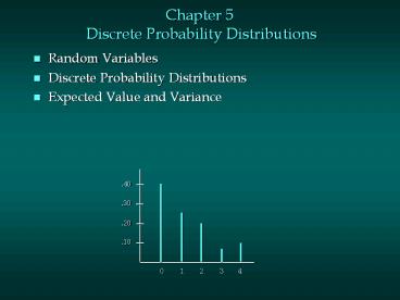
• Using past data on TV sales (below left), a
  tabular representation of the probability
  distribution for TV sales (below right) was
  developed.
• Number
• Units Sold of Days x f(x)
• 0 80 0 .40
• 1 50 1 .25
• 2 40 2 .20
• 3 10 3 .05
• 4 20 4 .10
• 200 1.00

7
Example JSL Appliances

• Graphical Representation of the Probability
  Distribution

.50
.40
Probability
.30
.20
.10
0 1 2 3 4
Values of Random Variable x (TV sales)
8
Discrete Uniform Probability Distribution

• The discrete uniform probability distribution is
  the simplest example of a discrete probability
  distribution given by a formula.
• The discrete uniform probability function is
• f(x) 1/N
• where
• N the number of values the random
• variable may assume
• Note that the values of the random variable are
  equally likely.

9
Expected Value and Variance

• The expected value, or mean, of a random variable
  is a measure of its central location.
• E(x) ? ?xf(x)
• The variance summarizes the variability in the
  values of a random variable.
• Var(x) ? 2 ?(x - ?)2f(x)
• The standard deviation, ?, is defined as the
  positive square root of the variance.

10
Example JSL Appliances

• Expected Value of a Discrete Random Variable
• x f(x) xf(x)
• 0 .40 .00
• 1 .25 .25
• 2 .20 .40
• 3 .05 .15
• 4 .10 .40
• E(x) 1.20
• The expected number of TV sets sold in a day is
  1.2

11
Example JSL Appliances

• Variance and Standard Deviation
• of a Discrete Random Variable
• x x - ? (x - ?)2 f(x) (x - ?)2f(x)
• 0 -1.2 1.44 .40 .576
• 1 -0.2 0.04 .25 .010
• 2 0.8 0.64 .20 .128
• 3 1.8 3.24 .05 .162
• 4 2.8 7.84 .10 .784
• 1.660 ? ?
• The variance of daily sales is 1.66 TV sets
  squared.
• The standard deviation of sales is 1.2884 TV
  sets.

12
Example XYZ Electronics

• The supervisor of XYZ would like to know what the
  average number of absentees is daily and also
  what the standard deviation is of the daily
  employee absentee rate. Historical data provides
  the follow probability distribution
• Daily
• Absentees f(x)
• 0 .50
• 1 .23
• 2 .12
• 3 .10
• 4 .02
• 5 .02
• 6 .01
• 1.00

13
Example XYZ Electronics

• Expected Value of a Discrete Random Variable
• x f(x) xf(x)
• 0 .50 .00
• 1 .23 .23
• 2 .12 .24
• 3 .10 .30
• 4 .02 .08
• 5 .02 .10
• 6 .01 .06
• E(x) 1.01
• The expected number of absentees is 1.01

14
Example XYZ Electronics

• Variance and Standard Deviation
• of a Discrete Random Variable
• x x - ? (x - ?)2 f(x) (x - ?)2f(x)
• 0 -1.01 1.0201 .50 .5101
• 1 -0.01 0.0001 .23 .0000
• 2 0.99 0.9801 .12 .1176
• 3 1.99 3.9601 .10 .3960
• 4 2.99 8.9401 .02 .1788
• 5 3.99 15.9201 .02 .3184
• 6 4.99 24.9001 .01 .2490
• 1.7699 ? ?
• The variance of absentees is 1.7699 squared.
• The standard deviation of absentees is
  1.3304.