Assumptions in linear regression models

1
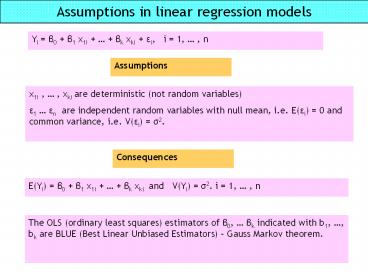
Assumptions in linear regression models
Yi ß0 ß1 x1i ßk xki ei, i 1, , n
Assumptions
x1i , , xki are deterministic (not random
variables) e1 en are independent random
variables with null mean, i.e. E(ei) 0 and
common variance, i.e. V(ei) s2.
Consequences
E(Yi) ß0 ß1 x1i ßk xki and V(Yi)
s2. i 1, , n
The OLS (ordinary least squares) estimators of
ß0, ßk indicated with b1, , bk are BLUE (Best
Linear Unbiased Estimators) Gauss Markov
theorem.
2
Normality assumption
If, in addition, we assume that the errors are
Normal r.v.
e1 en are independent NORMAL r.v. with null
mean and common variance s2, i.e. ei N(0, s2), i
1, , n
Consequences
Yi N( ß0 ß1 x1i ßk xki , s2), i 1,
, n
bi N( ßi V(bi)), i 0, , k
The normality assumption is needed to make
reliable inference (confidence intervals and
tests of hypotheses). I.e. probability statements
are exact If the normality assumption does not
hold, under some conditions, a large n
(observations), via a Central Limit theorem
allows reliable asymptotic inference on the
estimated betas.
3
Checking assumptions

• The error term e is unobservable. Instead we can
  provide an estimate by using the parameter
  estimates.
• The regression residual is defined as

?
ei yi yi , i 1, 2, ... n

• Plots of the regression residuals are fundamental
  in revealing model inadequacies such as
• non-normality
• unequal variances
• presence of outliers
• correlation (in time) of error terms

4
Detecting model lack of fit with residuals

• Plot the residuals ei on the vertical axis
  against each of the independend variables x1,
  ..., xk on the horizontal axis.
• Plot the residuals ei on the vertical axis
  against the predicted value y on the horizontal
  axis.
• In each plot look for trends, dramatic changes in
  variability, and /or more than 5 residuals lie
  outside 2s of 0. Any of these patterns indicates
  a problem with model fit.

?
Use the Scatter/Dot graph command in SPSS to
construct any of the plots above.
5
Examples residuals vs. predicted
fine
nonlinearity
unequal variances
outliers
6
Examples residuals vs. predicted
auto-correlation
nonlinearity and auto-correlation
7
Partial residuals plot

• An alternative method to detect lack of fit in
  models with more than one independent variable
  uses the partial residuals for a selected j-th
  independent var xj,

e y (b0 b1x1... bj-1xj-1 bj1xj1 ...
bkxk ) e bjxj
Partial residuals measure the influence of xj
after the effects of all other independent vars
have been removed. A plot of the partial
residuals for xj against xj often reveals more
information about the relationship between y and
xj than the usual residual plot. If everything
is fine they should show a straight line with
slope bj.
Partial residual plots can be calculated in SPSS
by selecting Produce all partial plots in the
Plots options in the Regression dialog box.
8
Example

• A supermarket chain wants to investigate the
  effect of price p on the weekly demand of a house
  brand of coffee.
• Eleven prices were randomly assigned to the
  stores and were advertised using the same
  procedure.
• A few weeks later the chain conducted the same
  experiment using no advertising

• Y weekly demand in pounds
• X1 price, dollars/pound
• X2 advertisement 1 Yes, 0 No.

Model 1 E(Y) ß0 ß1x1 ß2x2
Data Coffee2.sav
9
Computer Output
10
Residual and partial residual (price) plots
Residuals vs. price. Shows non-linearity
Partial residuals for price vs. price. Shows
nature of non-linearity. Try using 1/x instead of
x
11
E(Y) ß0 ß1(1/x1) ß2x2
RecPrice 1/Price
12
Residual and partial residual (1/price) plots
After fitting the independent variable x1
1/price the Residual plot does not show any
pattern and the Partial residual plot for
(1/price) does not show any non linearity.
13
An example with simulated data
The true model, supposedly unknown, is Y 1
x1 2x2 1.5x1x2 e, with eN(0,1)
Data Interaz.sav
Fit a model based on data
Fit a model based on data
X2
Cor(X1,X2)0.131
Y
x1
x2
14
Model 1 E(Y) ß0 ß1x1 ß2x2
Anovab Anovab Anovab Anovab Anovab Anovab Anovab
SS df MS F Sig.
Regressione 8447,42 2 4233,711 768,494 ,000a
Residuo 533,12 97 5,496
Totale 8980,54 99


Adj. R20.939
Coefficientia Coefficientia Coefficientia Coefficientia Coefficientia Coefficientia Coefficientia Coefficientia Coefficientia
t Sig.
B DS t Sig. VIF
1 (Costante) -6,092 ,630 -9,668 ,000
1 X1 3,625 ,207 17,528 ,000 1,018
1 X2 6,145 ,189 32,465 ,000 1,018

15
Model 1 standardized residual plot
Nonlinearity is present
To what is due?
Since the scatter-plots do not show any
non-linearity it could be due to an interaction
Y
16
Model 1 partial regression plots
Show that linear effects are roughly fine. But
some non-linearity shows up
X1
X2
17
Model 2 E(Y) ß0 ß1x1 ß2x2 ß3x1x2
Anovab Anovab Anovab Anovab Anovab Anovab Anovab
SS df MS F Sig.
Regressione 8885,372 3 2961,791 2987,64 000a
Residuo 95,169 96 ,991
Totale 8980,541 99


Adj. R20.989
Coefficientia Coefficientia Coefficientia Coefficientia Coefficientia Coefficientia Coefficientia Coefficientia Coefficientia
t Sig.
B DS t Sig. VIF
1 (Costante) ,305 ,405 ,753 ,453
1 X1 1,288 ,142 9,087 ,000 2,648
1 X2 2,098 ,209 10,051 ,000 6,857
1 IntX1X2 1,411 ,067 21,018 ,000 9,280

18
Model 2 standardized residual plot
Looks fine
19
Model 2 partial regression plots
Maybe an outlier is present
X1
X2
All plots show linearity of the corresponding
terms
X1X2
20
Model 3 E(Y) ß0 ß1x1 ß2x2 ß3x1x2
ß4x22
Suppose I wanto to try fitting a quadratic term
Anovab Anovab Anovab Anovab Anovab Anovab Anovab
SS df MS F Sig.
Regressione 8890,686 4 2222,67 2349,92 ,000a
Residuo 89,856 95 ,946
Totale 8980,541 99


Adj. R20.990
Coefficientia Coefficientia Coefficientia Coefficientia Coefficientia Coefficientia Coefficientia Coefficientia Coefficientia
t Sig.
B DS t Sig. VIF
1 (Costante) ,023 ,413 ,055 ,956
1 X1 1,258 ,139 9,051 ,000 2,670
1 X2 2,615 ,299 8,757 ,000 14,713
1 IntX1X2 1,436 ,066 21,619 ,000 9,528
1 X2Square -,137 ,058 -2,370 ,020 11,307

x22 seems fine
Higher MC
21
Model 3 standardized residual plot
Looks fine
22
Model 3 partial regression plots
X1
X2
Doesnt show linearity
X1X2
X22
23
Checking the normality assumption

• The inference procedures on the estimates (tests
  and confidence intervals) are based on the
  Normality assumption on the error term e. If this
  assumption is not satisfied the conclusions drawn
  may be wrong.

Again, the residuals ei are used for checking
this assumption

• Two widely used graphical tools are
• the P-P plot for Normality of the residuals
• the histogram of the residuals compared with the
  Normal density function.

The P-P plot for Normality and histogram of the
residuals can be calculated in SPSS by selecting
the appropriate boxes in the Plots options in
the Regression dialog box.
24
Social Workers example E(ln(Y)) ß0 ß1x
Points should be as close as possible to the
straight line
Histogram should match the continuous line

• Both graphs do not show strong departures from
  the Normality assumption.