Implementation Tasks

1
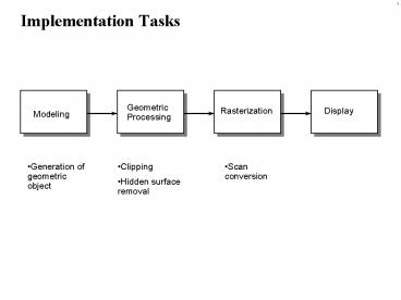
Implementation Tasks

• Clipping
• Hidden surface removal

• Generation of geometric object

• Scan conversion

2
Modeling

• Produces a set of vertices that specifies a set
  of geometric objects.
• The modeler that produces geometric objects is
  usually a user program with an interactive
  interface.

3
Geometric Processing

• Determine which geometric objects appear on the
  display.
• Assign shades or colors to these objects.
• Four related processes
• Normalization
• Clipping
• Hidden-surface removal
• Shading

4
Rasterization

• Convert vertices into a set of pixel values
  through scan conversion.
• Most scan conversion algorithms are designed for
  line segments and polygons.
• Other objects are rasterized by approximating
  them with line segments and polygons.

5
Display

• The process of taking the image from the frame
  buffer and displaying it on a CRT.
• Happens automatically and is not of concern to
  the application program.

6
Implementation Strategies
Object oriented for(each_object) render
(object) - Pipelined vertex oriented renderer
fits this strategy - Any primitive potentially
affects any set of pixels in the frame
buffer/z buffer Image oriented for
(each_pixel) assign_a_color (pixel) -
Generates pixels in the order required to refresh
the display. - Requires complex geometric
data structure
7
Transformation Sequence
Normalized Device Coords.
Screen Coords.
Clip Coords.
Object Coords.
Eye Coords.
Implementation 4 x 4 matrix multiplication in
homogeneous coords.
8
Clipping Against a Rectangular RegionMultiple
Cases
B
F
E
C
G
A
D
H
Clip Rectangle
9
Division of Space
Clip Region
10
Cohen-Sutherland ClippingOutcodes
11
Cohen-Sutherland ClippingRegion Outcodes
1001
1000
1010
0001
0010
0000
0100
0110
0101
12
Cohen-Sutherland ClippingTrivial Acceptance
O(P0) O(P1) 0
1001
1000
1010
P1
0001
0010
0000
P0
0100
0110
0101
13
Cohen-Sutherland ClippingTrivial Rejection
O(P0) O(P1) ? 0
P0
1001
1000
1010
P1
P0
0001
0010
0000
P0
P1
P1
0100
0110
0101
14
Cohen-Sutherland Clipping O(P0) 0 , O(P1) ? 0
1001
1000
1010
P0
0001
0010
0000
P1
P1
P0
P0
0100
0110
0101
P1
15
Cohen-Sutherland Clipping O(P0) O(P1) 0
1001
1000
1010
P0
P1
0001
0010
0000
0100
0110
0101
16
Cohen-Sutherland ClippingOutside vs. Inside
1001
1000
1010
0001
0010
0000
0100
0110
0101
Inside
17
Cohen-Sutherland Clipping The Algorithm

• Compute the outcodes for the two vertices
• Test for trivial acceptance or rejection
• Select a vertex for which outcode is not zero
• There will always be one
• Select the first nonzero bit in the outcode to
  define the boundary against which the line
  segment will be clipped
• Compute the intersection and replace the vertex
  with the intersection point
• Compute the outcode for the new point and iterate

18
Cohen-Sutherland ClippingExample 1
A
1001
1000
1010
B
C
0001
0010
0000
0100
0110
0101
19
Cohen-Sutherland ClippingExample 1
1001
1000
1010
B
C
0001
0010
0000
0100
0110
0101
20
Cohen-Sutherland ClippingExample 2
1001
1000
1010
E
D
0001
0010
0000
C
B
A
0100
0110
0101
21
Cohen-Sutherland ClippingExample 2
1001
1000
1010
E
D
0001
0010
0000
C
B
0100
0110
0101
22
Cohen-Sutherland ClippingExample 2
1001
1000
1010
D
0001
0010
0000
C
B
0100
0110
0101
23
Cohen-Sutherland ClippingExample 2
1001
1000
1010
0001
0010
0000
C
B
0100
0110
0101
24
Cohen-Sutherland ClippingAdvantages/Extension

• Easily extended to 3 dimensions by adding two
  bits to the outcode for the z axis.
• Calculations then reduce to intersection of line
  with plane
• Algorithm most efficient when most segments can
  either be trivially accepted or trivially rejected

You may like to try out the Clipping Applet to
see the effect of Cohen-Sutherland clipping.
25
Parametric Representation of Lines
26
Liang-Barsky Parametric Clipping
Edge Ei
Inside
Outside
27
Potentially Entering (PE) and Potentially Leaving
(PL) Points
Edge Ei
Edge Ei
Inside
Outside
Inside
Outside
Potentially Entering (PE) Point
Potentially Leaving (PL) Point
28
Liang-Barsky ClippingComputing the Intersection
29
Liang-Barsky ClippingPotentially Leaving vs.
Potentially Entering
PE
PL
PL
PL
PE
PL
PE
PE
Inside
30
Liang-Barsky ClippingAlgorithm Strategy

• Find the largest PE greater than zero.
• Find the smallest PL less than one.
• Reject the segment if PE gt PL.

31
Liang-Barsky ClippingPseudocode of Algorithm
for (each line segment to be clipped) alpha_E0
alpha_L1 for (each candidate intersection with
a clip edge) if (NiD!0) /edges not
parallel to line/ calculate alpha use
sign of NiD to class alpha as PE or PL if
(PE) alpha_E max(alpha_E,alpha) if (PL)
alpha_L min(alpha_L,alpha) if (alpha_E
gt alpha_L) return NULL else return
P(alpha_E) and P(alpha_L) as clip intersections
32
Sutherland-Hodgeman Pipeline Clipping
33
Polygon ClippingConvex Polygons
5
4
4
5
1
3
1
3
2
2
Line segment clipping is done in order. New
vertices are generated at clip point. External
vertices are eliminated.
34
Polygon ClippingThe Convexity Problem
Single object becomes multiple objects.
35
Sutherland-Hodgeman Polygon Clipping
36
Hidden Surface Removal

• Given a set of geometric entities, the
  hidden-surface removal algorithm determines
• whether object is visible to the viewer,
• whether object is obscured from the viewer by
  other objects.

37
Object-Space Approach

• Pick one of the k polygons in the scene.
• Compare it pairwise with the remaining k-1
  polygons.
• Complexity of the algorithm
• The approach works best for scenes with
  relatively few polygons.

38
Image-Space Approach

• Intersect a cast ray from the center of
  projection with each of the k polygons.
• Find the intersection closest to the center of
  projection.
• Color the current pixel with the shade of this
  polygon.
• Complexity of the algorithm

39
Back-Face Removal

• In situations where we cannot see the back-facing
  polygons, we can eliminate them before applying
  hidden surface removal.
• The front of the polygon can be seen if
• We can use the dot product to test this condition

40
Z-Buffer Algorithm

• Most widely used hidden surface removal
  algorithm.
• Easy to implement in either hardware or software.
• Works in image space but loops over the polygons
  rather than pixels.

41
Example

• Cast a ray from COP and intersect with all
  polygons.
• Point on a polygon is visible if it is the
  closest point of intersection along the ray.
• Since , points on B will appear
  on the screen.
• Points on A will not appear on the screen.

42
The Algorithm

• Initialize
• Each z-buffer location ? max z value.
• Each frame buffer location ? background color.
• For each polygon
• Compute z(x,y), polygon depth at the pixel (x,y).
• If z(x,y)ltz-buffer value at pixel (x,y) then
• Z-buffer(x,y) ? z(x,y)
• Pixel(x,y)?color of polygon at (x,y).

43
Calculation of Z value

• For the same scan line, the above equation becomes

44
The Rasterization Problem Idealized
PrimitivesMap to Discrete Display Space
45
Solution Involves Selection of DiscreteRepresenta
tion Values
46
Scan Converting LinesCharacterizing the Problem
ideal line
i.e. for each x, choose y
i.e. for each y, choose x
47
Scan Converting LinesThe Strategy

• Pick pixels closest to endpoints
• Select in between pixels closest to ideal line
• Objective To minimize the required calculations.

48
Scan Converting LinesDDA (Digital Differential
Analyzer) Algorithm
Selected
Not Selected
49
Scan Converting LinesDDA Algorithm, Incremental
Form
Therefore, rather than recomputing y in each
step, simply add m.
The Algorithm
void Line(int x0, int y0, int xn, int yn) int
x float dy, dx, y, m dy yn - y0 dx xn -
x0 m dy/dx y y0 for (x x0
xltxn,x) WritePixel(x, round(y)) y
m
50
Bresenhams AlgorithmAllowable Pixel Selections
Not Allowed
Option NE
0 lt Slope lt 1
Option E
Last Selection
51
Bresenhams AlgorithmIterating
0 lt Slope lt 1
Select E
Select NE
52
Bresenhams AlgorithmDecision Function
(implicit equation of the line)
53
Bresenhams AlgorithmCalculating the Decision
Function
54
Bresenhams AlgorithmIncremental Calculation of
di
55
Bresenhams AlgorithmThe Code
void BresenhamLine(int x0, int y0, int xn, int
yn) int dx,dy,incrE,incrNE,d,x,y dxxn-x0
dyyn-y0 d2dy-dx / initial value of d
/ incrE2dy / decision funct incr for
E / incrNE2dy-2dx / decision funct incr
for NE / xx0 yy0 DrawPixel(x,y) /
draw the first pixel / while (xltxn) if
(dlt0) / choose E / dincrE x
/ move E / else / choose
NE / dincrNE x y /
move NE / DrawPixel (x,y)
56
Bresenhams AlgorithmAn example
12
11
10
9
8
7
4
5
6
7
8
9
57
Bresenhams AlgorithmAn example
12
11
10
9
8
7
4
5
6
7
8
9
58
Bresenhams AlgorithmAn example
12
11
10
9
8
7
4
5
6
7
8
9
59
Filling PolygonsScan Line Algorithm
14
12
10
8
6
4
2
0
2
4
6
8
10
12
14
0
60
Filling PolygonsScan Line Algorithm

• 1. Find the intersections of current scan line
  with all edges of the
• polygon.
• 2. Sort the intersections by increasing x
  coordinate.
• 3. Fill in pixels that lie between pairs of
  intersections that lie
• interior to the polygon using the odd/even
  parity rule.

61
Filling PolygonsSpecial Cases
Edge Table (ET) Entry
62
Scan Line Polygon Fill Algorithm
N
N
14
N
D
12
N
EF
DE
F
10
-5/2
6/4
N
9
7
12
7
CD
N
8
N
12
13
0
E
6
C
FA
N
4
N
9
2
0
A
2
N
AB
BC
B
0
6/4
N
7
-5/2
3
7
5
2
4
6
8
10
12
14
0
N
Scan Line
63
Scan Line Polygon FillThe Algorithm

• Set y to smallest y coordinate that has an entry
  in ET
• Initialize the active edge table (AET) to empty
• Repeat until the ET and AET are both empty
• Move from ET bucket at y to AET those edges whose
  ymin y. (entering edges)
• Remove from AET those edges for which y ymax.
• Sort AET on x
• Fill in desired pixels on scan line using
  even-odd parity from AET
• Increment y by one (next scan line)
• For each edge in the AET, update x by adding Dx/Dy