Numerical Solution to Differential Equations

1
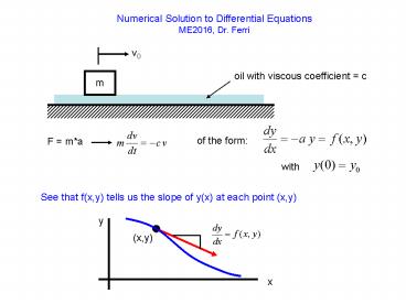
Numerical Solution to Differential
Equations ME2016, Dr. Ferri
v0
oil with viscous coefficient c
m
of the form
F ma
with
See that f(x,y) tells us the slope of y(x) at
each point (x,y)
y
(x,y)
x
2
Vector Field for
Exact soln., y0 6
Exact soln., y0 4
Exact soln., y0 2
3
Taylor Series Analysis
v0
oil with viscous coefficient c
m
F ma
of the form
with
Could expand y(x) in a Taylor series
or
4
In general, letting
and
1st-order Euler Integration? drop higher-order
terms
More-accurate algorithms can be developed, based
on keeping more and more terms in the Taylor
series.
5
Alternate Approach
v0
oil with viscous coefficient c
m
of the form
F ma
with
Integrate over small time interval, h
6
In general,
The problem is that we dont know y(x), so
evaluating the integral is not trivial.
Could assume that if h is small enough, f(x,y)
will not change that much over the integral.
Using left-rectangular integration,
This may be recognized as 1st-order Euler
Integration. A family of improved versions are
terms Runge-Kutta methods
7
Runge-Kutta Methods
1st-order Euler prediction
y
yi
true solution
h
x
xi
xi1 xi h
Tuncation error
true solution
8
Runge-Kutta Methods
1st-order Euler prediction yi1
y
yi
true solution
fi
h
x
xi
xi1 xi h
Various RK methods differ in how they estimate fi
For 1st-order Euler integration, fi f(xi, yi)
9
2nd-order RK
y
yi
fi
h
average of two slopes
x
xi
xi1 xi h
Error is lower than Euler, but now there are 2
calls to f(x,y) required per step
Tuncation error
true solution
10
2nd-order RK Algorithm
predictor
corrector
11
Huens Method
predictor
iteration
corrector
12
4th-order RK
weighted average
where
different estimates of slope
13
ERRORS
Local (single-step)
Global (multi-step)
function evals per step
RK
1st-order
1
O(h2)
O(h) O(1/n)
2nd-order
O(h3)
O(h2) O(1/n2)
2
4th-order
O(h5)
O(h4) O(1/n4)
4
local error
For n steps,
Therefore, global error
Order of global error is 1 less than order of
local error
14
A fair comparison between two RK methods must
account the differing number of function calls
per step
RK1 (Euler-integration)- - 1 function call per
step
x0
x1
x2
x3
x4
x5
x8
x6
x7
RK4 - - 4 function calls per step
x0
x1
x2
Example integrate from 0 to 4 using n400
function evaluations
1st-order Euler with h 0.01 global error
O(0.01)
4th-order RK with h 0.04 global error
O(0.00000256)
104 times less error for same amount of work ?
FREE LUNCH !!!
15
v0
oil with viscous coefficient c
m
F ma
of the form
a1 v0 2 h0.1 n 10 yi v0 Y(1)
yi xi0 X(1)xi for i 1n xi (i-1)h
fi -ayi yip1 yi fih xip1 xi
h Y(i1)yip1 X(i1)xip1 yi
yip1 end
plot(X,Y,'o-',X,v0exp(-aX),'r-') xlabel('Time')
ylabel('Speed') legend('Euler, h 0.1','Exact')
16
(No Transcript)
17
1st-order Euler Method Detail of comparison of h
0.1 with h 0.05
See that halving h cuts the error in half
(approximately)
18
Example, 2nd-order RK
and
Exact solution
The numerical algorithm is unstable because h is
too large !
19
Reducing h to 0.2 gives a stable, accurate
algorithm
20
Higher-order systems of equations
Predator-prey problem let y1 the number of
rabbits
let y2 the number of foxes
Governing equations
,
or
In vector form
1st-order Euler
21
Create a m-file function pprey.m
function yprime pprey(t,y) a 1.2 b0.6
c0.8 d0.3 yprime(1)ay(1)-by(1)y(2) yprim
e(2)-cy(2)dy(1)y(2) yprimeyprime()
h0.001 n 30000 yi 2 1 Y(,1)
yi ti0 T(1)ti for i 1n ti (i-1)h
fi pprey(ti,yi) yip1 yi fih tip1
ti h Y(,i1)yip1 T(i1)tip1 yi
yip1 end plot(T,Y(1,),'-',T,Y(2,),'--') xlab
el('Time') ylabel('Population') legend('Rabbits',
'Foxes')
vv() just makes v a column vector
22
(No Transcript)
23
Can also generate a phase plot of foxes vs
rabbits
24
Built-in Matlab RK Programs
Vector of initial conditions
Timespan t0 tf
String containing the name of the m-file that
calculates yprime
t,y ode45('pprey',0 30,2 1)
time
Matlab function for 4th and 5th-order RK
Matrix of response 1st-col y1, 2nd-coly2, etc
other ODE solvers ODE23, ODE113, ODE15S,
ODE23S, ODE23T, ODE23TB