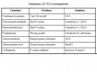
Summary of OLS assumptions

1
Summary of OLS assumptions
2
Model specification errors

• Including irrelevant terms
• Parameter estimates unbiased
• P-values too large
• Failing to incorporate relevant terms
• Parameter estimates biased

• Our questions are usually framed in the context
  of all else equal
• Important to include control variables that may
  not be equal
• Dummies for observer, lab
• Social variables income, political attitudes,
  population size
• Physical variables temperature, slope, latitude

3
What if our data dont support our scientific
model?

• We are failing to account for important control
  variables
• Think about what factors might be influencing our
  results
• Collect data on them, and include them in the
  model
• The level of natural variability in our system is
  large
• If there are no control variables for this
  variability, then we need to increase the sample
  size
• Our scientific model might be wrong!

4
Outliers, leverage, and influence

• Outliers data points with unusually large
  residuals
• If residuals are normally distributed, only about
  5 of points should have studentized residuals
  with absolute values greater than 2
• Leverage points further from the mean of the X
  values have greater pull on the regression line
• Hat values greater than 2 or 3 times the average
  are considered unusual

• Influence A data point has large influence if
  deleting that point substantially changes the
  parameter estimates
• Influence depends both on outlyingness and
  leverage
• Cooks D provides a measure of influence
• Values greater than 4/(n-k-1) considered large (n
  is number of points, k is number of coefficients)

5
(No Transcript)
6
What can we do about chlorophyll regression?

• Square root transform helps a little with
  non-normality and a lot with heteroskedasticity

• But it makes nonlinearity worse

7
A new model
Call lm(formula Chlorophyll.pow
sqrt(Phosphorus) sqrt(NP)) Residuals Min
1Q Median 3Q Max -1.5846 -0.7758
-0.1640 0.6975 2.5464 Coefficients
Estimate Std. Error t value Pr(gtt)
(Intercept) -0.90141 0.61584 -1.464
0.157414 sqrt(Phosphorus) 0.21408 0.09547
2.242 0.035348 sqrt(NP) 0.15133
0.03742 4.044 0.000542 --- Signif. codes
0 ' 0.001 ' 0.01 ' 0.05 .' 0.1 ' 1
Residual standard error 1.198 on 22 degrees of
freedom Multiple R-Squared 0.897, Adjusted
R-squared 0.8876 F-statistic 95.77 on 2 and 22
DF, p-value 1.388e-11
8
(No Transcript)
9
(No Transcript)
10
R code, part 1

• Read in the data
• chlor lt- read.csv("Chlorophyll.csv")
• attach(chlor)
• Run our regression from before
• chlor1.lm lt- lm(Chlorophyll.a Phosphorus
  PhosphorusNitrogen)
• Look at influence, outlyingness, and leverage
  of points
• influence.plot(chor1.lm)
• Re-run the transformed model, and look at the
  CR plots
• NP lt- NitrogenPhosphorus
• chlor4.lm lt- lm(Chlorophyll.pow Phosphorus
  NP)
• cr.plots(chlor4.lm, askF)

11
R code, part 2

• Now fit a model with the independent variables
  also transformed, and look at the diagnostics
• chlor5.lm lt- lm(Chlorophyll.pow
  sqrt(Phosphorus) sqrt(NP))
• summary(chlor5.lm)
• cr.plots(chlor5.lm, askF)
• qq.plot(rstudent(chlor5.lm))
• plot(fitted(chlor5.lm),rstudent(chlor5.lm))
• abline(0,0,lty3)