Graphs Traversals

1
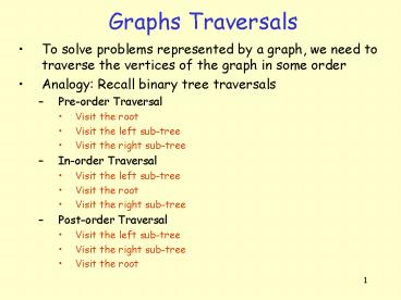
Graphs Traversals

• To solve problems represented by a graph, we need
  to traverse the vertices of the graph in some
  order
• Analogy Recall binary tree traversals
• Pre-order Traversal
• Visit the root
• Visit the left sub-tree
• Visit the right sub-tree
• In-order Traversal
• Visit the left sub-tree
• Visit the root
• Visit the right sub-tree
• Post-order Traversal
• Visit the left sub-tree
• Visit the right sub-tree
• Visit the root

2
Graph Traversals

• Traversing trees is easy since trees have a nice
  structure and are acyclic graphs
• What about graphs which have arbitrary topology?
• 2 traversal (search) methods
• Breath-first search
• Starting at a node visit ALL of your neighbors
• Then visit the neighbors of your neighbors and so
  on
• Like a wave-front expanding outwards from a
  source node
• Depth-first search
• Starting at a node, follow a path all the way
  until you cannot move any further
• Then backtrack and try another branch
• Do this until all nodes have been visited

3
Breath-First Search - Idea
2
1
2
2
s
s
s
1
2
2
1
2

• Given a graph G (V, E), start at the source
  vertex s and discover which vertices are
  reachable from s
• At any time there is a frontier of vertices
  that have been discovered, but not yet processed
• Next pick the nodes in the frontier in sequence
  and discover their neighbors, forming a new
  frontier
• Breadth-first search is so named because it
  visits vertices across the entire breadth of this
  frontier before moving on

4
BFS - Continued

• Represent the final result as follows
• For each vertex v e V, we will store dv which
  is the distance (length of shortest path) from s
  to v
• Distance between a vertex v and s is defined
  to be the minimum number of edges on a path from
  s to v
• Note that ds 0
• We will also store a predecessor (or parent)
  pointer predv or pv, which indicates the
  first vertex along the shortest path if we walk
  from v backwards to s
• We will let prevs or ps 0
• Notice that these predecessor pointers are
  sufficient to reconstruct the shortest path to
  any vertex

5
BFS Implementation
2
1
2
2
s
s
s
1
2
2
1
2

• Initially all vertices (except the source) is
  colored white, meaning they have not been
  discovered just yet
• When a vertex is first discovered, it is colored
  gray (and is part of the frontier)
• When a gray vertex is processed, it becomes black

6
BFS - Implementation
2
1
2
2
s
s
s
1
2
2
1
2

• The search makes use of a FIFO queue, Q
• We also maintain arrays
• coloru, which holds the color of vertex u
• either white, gray, black
• predu, which points to the predecessor of u
• The vertex that discovered u
• du, the distance from s to u

7
BFS Implementation

• BFS(G, s)
• for each u in V- s
  // Initialization
• coloru white
• du INFINITY
• predu NULL
• //end-for
• colors GRAY
  // initialize source s
• ds 0
• preds NULL
• Q s
  // Put s in the queue
• while (Q is nonempty)
• u Dequeue(Q)
  // u is the next vertex to visit
• for each v in Adju
• if (colorv white)
  // if neighbor v undiscovered
• colorv gray
  // mark is discovered
• dv du 1
  // set its distance
• predv u
  // set its predecessor

8
BFS - Example
w
w
v
u
v
u
w
u
v
i
2
i
1
1
i
i
2
i
i
i
0
0
i
0
1
1
i
t
t
s
s
t
s
x
x
x
Q v, x
Q x, u, w
Q s
w
v
u
w
v
u
w
v
u
2
1
2
2
1
2
2
1
2
i
0
1
3
0
t
s
1
3
x
0
1
t
s
x
t
s
x
Q u, w
Q w, t
Q
9
BFS - Analysis

• Let n V and e E
• Observe that the initial portion requires q(n)
• The real meat is through the traversal loop
• Since we never visit a vertex twice, the number
  of times we go through the loop os at most n
  (exactly n assuming each vertex is reachable from
  the source)
• The number of iterations through the inner loop
  is proportional to deg(u)
• Summing up over all vertices we have
• T(n) n Sum_v e V degv n 2e q(ne)

10
BFS Tree
s
0
w
v
u
v
x
1
1
2
1
2
u
w
2
2
3
0
1
t
x
t
3

• The predecessor pointers of the BFS define an
  inverted tree
• If we reverse these edges, we get a rooted,
  unordered tree called a BFS tree for G
• There are many potential BFS trees for a graph
  depending on where the search starts and in what
  order vertices are placed on the queue
• These edges of G are called the tree edges, and
  the remaining edges are called the cross edges

11
BFS Tree
s
0
w
v
u
v
x
1
1
2
1
2
u
w
2
2
3
0
1
t
x
t
3

• It is not hard to prove that if G is an
  undirected graph, then cross edges always go
  between two nodes that are at most ONE level
  apart in the BFS tree
• The reason is that if any cross edge spanned two
  or more levels, then when the vertex at the
  higher level (closer to the root) was being
  processed, it would have discovered the other
  vertex, implying that the other vertex would
  appear on the next level of the tree, a
  contradiction
• In a directed graph, cross edges may come up at
  an arbitrary number of levels