Real GDP with a Fixed Price Level

1
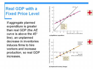
Real GDP with aFixed Price Level

• If aggregate planned expenditure is greater than
  real GDP (the AE curve is above the 45 line), an
  unplanned decrease in inventories induces firms
  to hire workers and increase production, so real
  GDP increases.

2
Real GDP with aFixed Price Level

• If aggregate planned expenditure is less than
  real GDP (the AE curve is below the 45 line), an
  unplanned increase in inventories induces firms
  to fire workers and decrease production, so real
  GDP decreases.

3
Real GDP with aFixed Price Level

• If aggregate planned expenditure equals real GDP
  (the AE curve intersects the 45 line), no
  unplanned changes in inventories occur, so firms
  maintain their current production and real GDP
  remains constant.

4
The Multiplier

• The multiplier is the amount by which a change in
  autonomous expenditure is magnified or multiplied
  to determine the change in equilibrium
  expenditure and real GDP.

5
The Multiplier

• The Basic Idea of the Multiplier
• An increase in investment (or any other component
  of autonomous expenditure) increases aggregate
  expenditure and real GDP and the increase in real
  GDP leads to an increase in induced expenditure.
• The increase in induced expenditure leads to a
  further increase in aggregate expenditure and
  real GDP.
• So real GDP increases by more than the initial
  increase in autonomous expenditure.

6
The Multiplier

• Figure 29.7 illustrates the multiplier.
• The Multiplier Effect
• The amplified change in real GDP that follows an
  increase in autonomous expenditure is the
  multiplier effect.

7
The Multiplier

• When autonomous expenditure increases,
  inventories make an unplanned decrease, so firms
  increase production and real GDP increases to a
  new equilibrium.

8
The Multiplier

• Why Is the Multiplier Greater than 1?
• The multiplier is greater than 1 because an
  increase in autonomous expenditure induces
  further increases in expenditure.
• The Size of the Multiplier
• The size of the multiplier is the change in
  equilibrium expenditure divided by the change in
  autonomous expenditure.

9
The Multiplier

• The Multiplier and the Marginal Propensities to
  Consume and Save
• Ignoring imports and income taxes, the marginal
  propensity to consume determines the magnitude of
  the multiplier.
• The multiplier equals 1/(1 MPC) or,
  alternatively, 1/MPS.

10
The Multiplier

• Figure 29.8 illustrates the multiplier process
  and shows how the MPC determines the magnitude of
  the amount of induced expenditure at each round
  as aggregate expenditure moves toward equilibrium
  expenditure.

11
The Multiplier Math

• ?Y ?I b?I b2?I b3?I b4?I b5?I .
• Multiply by b to obtain
• b?Y b?I b2?I b3?I b4?I b5?I .
• bn approaches zero as n becomes large so b(n 1)
  also approaches zero.
• Subtract the second equation from the first to
  obtain
• ?Y b?Y ?I, or (1 b) ?Y ?I,
• so that
• ?Y ?I/(1 b).

12
The Multiplier

• Imports and Income Taxes
• Income taxes and imports both reduce the size of
  the multiplier.
• Including income taxes and imports, the
  multiplier equals 1/(1 slope of the AE curve).

13
The Multiplier

• Figure 29.9 shows the relation between the
  multiplier and the slope of the AE curve.
• In part (a) the slope of the AE curve is 0.75 and
  the multiplier is 4.

14
The Multiplier

• In part (b) the slope of the AE curve is 0.5 and
  the multiplier is 2.

15
The Multiplier

• Business Cycle Turning Points
• Turning points in the business cyclepeaks and
  troughsoccur when autonomous expenditure
  changes.
• An increase in autonomous expenditure brings an
  unplanned decrease in inventories, which triggers
  an expansion.
• A decrease in autonomous expenditure brings an
  unplanned increase in inventories, which triggers
  a recession.

16
The Multiplier and the Price Level

• In the equilibrium expenditure model, the price
  level is constant.
• But real firms dont hold their prices constant
  for long.
• When they have an unplanned change in
  inventories, they change production and prices.
• And the price level changes when firms change
  prices.
• The aggregate supply-aggregate demand model
  explains the simultaneous determination of real
  GDP and the price level.
• The two models are related.

17
The Multiplier and the Price Level

• Aggregate Expenditure and Aggregate Demand
• The aggregate expenditure curve is the
  relationship between aggregate planned
  expenditure and real GDP, with all other
  influences on aggregate planned expenditure
  remaining the same.
• The aggregate demand curve is the relationship
  between the quantity of real GDP demanded and the
  price level, with all other influences on
  aggregate demand remaining the same.

18
The Multiplier and the Price Level

• Aggregate Expenditure and the Price Level
• When the price level changes, a wealth effect and
  substitution effect change aggregate planned
  expenditure and change the quantity of real GDP
  demanded.
• Figure 29.10 on the next slide illustrates the
  effects of a change in the price level on the AE
  curve, equilibrium expenditure, and the quantity
  of real GDP demanded.

19
The Multiplier andthe Price Level

• In Figure 29.10(a), a rise in price level from
  105 to 125 shifts the AE curve from AE0 downward
  to AE1 and decreases the equilibrium level of
  real output from 10 trillion to 9 trillion.

20
The Multiplier andthe Price Level

• In Figure 29.10(b), the same rise in the price
  level that lowers equilibrium expenditure, brings
  a movement along the AD curve to point A.

21
The Multiplier andthe Price Level

• A fall in price level from 110 to 85 shifts the
  AE curve from AE0 upward to AE2 and increases
  equilibrium real GDP from 10 trillion to 11
  trillion.

22
The Multiplier andthe Price Level
A fall in price level from 110 to 85 shifts the
AE curve from AE0 upward to AE2 and increases
equilibrium real GDP from 10 trillion to 11
trillion.
The same fall in the price level that raises
equilibrium expenditure brings a movement along
the AD curve to point C.
23
The Multiplier andthe Price Level

• Points A, B, and C on the AD curve correspond to
  the equilibrium expenditure points A, B, and C at
  the intersection of the AE curve and the 45 line.

24
The Multiplier andthe Price Level

• Figure 29.11 illustrates the effects of an
  increase in autonomous expenditure.
• An increase in autonomous expenditure shifts the
  aggregate expenditure curve upward and shifts the
  aggregate demand curve rightward by the
  multiplied increase in equilibrium expenditure.

25
The Multiplier andthe Price Level

• Equilibrium Real GDP and the Price Level
• Figure 29.12 shows the effect of an increase in
  investment in the short run when the prices level
  changes and the economy moves along its SAS curve.

26
The Multiplier andthe Price Level

• The increase in investment shifts the AE curve
  upward

and shifts the AD curve rightward.
With no change in the price level real GDP would
increase to 12 trillion at point B.
27
The Multiplier andthe Price Level

• The AD curve shifts rightward by the amount of
  the multiplier effect but equilibrium real GDP
  increases by less than this amount because the
  price level rises.

28
The Multiplier andthe Price Level

• Real GDP increases from 10 trillion from 11.3
  trillion, instead of to 12 trillion as it does
  with a fixed price level.

29
The Multiplier andthe Price Level

• Figure 29.13 illustrates the long-run effects of
  an increase in autonomous expenditure at full
  employment.

30
The Multiplier andthe Price Level

• If the increase in autonomous expenditure takes
  real GDP above potential GDP.
• The money wage rate rises, the SAS curve shifts
  leftward, and real GDP decreases until it is back
  at potential real GDP.
• The long-run multiplier is zero.