Types of classical controllers

1
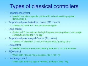
Types of classical controllers

• Proportional control
• Needed to make a specific point on RL to be
  closed-loop system dominant pole
• Proportional plus derivative control (PD control)
• Needed to bend R.L. into the desired region
• Lead control
• Similar to PD, but without the high frequency
  noise problem max angle contribution limited to
  lt 75 deg
• Proportional plus Integral Control (PI control)
• Needed to eliminate a non-zero steady state
  tracking error
• Lag control
• Needed to reduce a non-zero steady state error,
  no type increase
• PID control
• When both PD and PI are needed, PID PD PI
• Lead-Lag control
• When both lead and lag are needed, lead-lag
  lead lag

2
Proportional control design

• Draw R.L. for given plant
• Draw desired region for poles from specs
• Pick a point on R.L. and in desired region
• Use ginput to get point and convert to complex
• Compute
• Obtain closed-loop TF
• Obtain step response and compute specs
• Decide if modification is needed

nump denp sysptf(nump, denp)
rlocus(sysp)
x,yginput(1) pdxjy
Gpdevalfr(sysp,pd) K1/Gpd sysc K
syscl feedback(syscsysp,1)
use your program from several weeks ago to do all
these
3
PD controller design

• Design steps
• From specs, draw desired region for pole.Pick
  from region, not on RL
• Compute
• Select
• Select

x,yginput(1) pdxjy
Gpdevalfr(sysp,pd) phipi - angle(Gpd)
zabs(real(pd))abs(imag(pd)/tan(phi))
Kd1/abs(pdz)/abs(Gpd) KpzKd
4

• Approximation to PD
• Same usefulness as PD

• Lead Control
• Draw R.L. for G
• From specs draw region for desired c.l. poles
• Select pd from region
• LetPick z somewhere below pd on Re
  axisLetSelect

x,yginput(1) pdxjy
Gpdevalfr(sysp,pd) phipi - angle(Gpd)
x,yginput(1) zabs(x) phi1angle(pdz)
phi2phi1-phi
pabs(real(pd))abs(imag(pd)/tan(phi2))
Kabs((pdp)/(pdz)/Gpd)
sysctf(K1 z,1 p) Hold on rlocus(syscsysp)

5

• Alternative Lead Control
• Draw R.L. for G
• From specs draw region for desired c.l. poles
• Select pd from region
• Let
• Select

phipdangle(pd) phi1(phipdphi)/2
phi2phi1-phi
6
Lag Design steps

1. Draw R.L. for G(s).
2. From specs, draw desired pole region
3. Select pd on R.L. in region
4. Get
5. With that K, compute error constant(Kpa, Kva,
   Kaa) from KG(s)
6. From specs, compute Kpd, Kvd, Kad

sysol syscsysp nol, doltfdata(sysol,'v') d
n0dol(dol0) Kactnol(end)/dn0(end)
Kdes 1/ess
7

1. If Ka gt Kd , doneelse pick
2. Re-compute
3. Closed-loop simulation tuning as necessary

z-real(pd)/
pzKact/Kdes/(1)
0.05 or 0.1
8
PI Design steps

• First design design PD for G(s)/s
• Second design
• Draw R.L. for G(s)
• From specs, draw desired region
• Pick pd on R.L. in region
• i. Chooseii. Choose
• Simulate tune

9
Alternative PI design

• Since PI PD/s,
• Can first multiply system by 1/s
• Then design using PD, lead, lag
• The overall controller is the controller you
  designed divided by s

10

• Example
• Want
• Solution

C(s)
11
(No Transcript)
12

• Draw R.L.
• Pick pd on R.L. in Region pick pd 0.35
  j0.5
• Since there is one in G(s)

13
(No Transcript)
14
(No Transcript)
15
(No Transcript)
16
New root locus RL going north-east, ? reduce K
will increase s and
and increase z
17
Use original K0.86 instead of 0.914 ess should
be OK
Mp reduced by not enough.
18
Change that divide from 5 to 15.
ans yss1 ess0 tr2.78 td2.78 ts10.6
tp6.94 Mp15.8
19

• Lag control can improve ess, but cannot eliminate
  ess
• Use PI control to eliminate ess
• PI

20
Overall controller design
C(s)
Gp(s)
R(s)
E(s)
Y(s)
U(s)

1. Draw R.L. for G(s), hold graph
2. Draw desired region for closed-loop poles based
   on desired specs
3. If R.L. goes through region, pick pd on R.L. and
   in region. Go to step 7.

21

1. Pick pd in region (near corner but inside region
   for safety margin)
2. Compute angle deficiency
3. a. PD control, choose zpd such that then

22

1. b. Lead control choose zlead, plead such
   thatYou can select zlead compute plead. Or
   you can use the bisection method to compute z
   and p. Then

23

1. Compute overall gain
2. If there is no steady-state error requirement, go
   to 14.
3. With K from 7, evaluate error constant that you
   already have

24
The 0, 1, 2 should match p, v, a This is for
lag control. For PI
25

1. Compute desired error const. from specs
2. For PI set Ka Kd solve for zpiFor
   lag pick zlag let

26

1. Re-compute K
3. Get closed-loop T.F. Do step response analysis.
4. If not satisfactory, go back to 3 and redesign.

27
If we have both PI and PD we have PID control
28
If we have both Lead and Lag, we have lead-lag
control
29
Control System Implementation
C(s)
Gp(s)
R(s)
E(s)
Y(s)
U(s)
disturbance input
Reference Command
output
error
Controller
Actuator
control
Plant

plant input
_
Sensor
noise
30
PC-in-the-loop Control
disturbance input
Reference Command
PC I/O I/O
output
power Amp
Actuator
Plant
D/A
Signal Conditioner and amplifier
Sensor
A/D
All control algorithms implemented in PC (could
be Matlab Real-Time) Needs data acquisition
system, including A/D and D/A Needs power
amplifier
31
m-Controller based control
disturbance input
Reference Command
m-Controller I/O I/O
output
power Amp
Actuator
Plant
Signal Conditioner and amplifier
Sensor
Very similar architecture to PC-in-the-loop
control All control algorithms implemented in
m-controller m-controller has its own A/D and
D/A, but make sure resolution is OK Still needs
power amplifier, because m-controller outputs
weak signal
32
Power electronic based control
disturbance input
Reference Command
Difference amplifier
output
Op Amp circuit
Actuator
Plant
Sensor
Analog operation, fast Inexpensive All algorithms
in circuit hardware No sampling and aliasing
issues