
Topic 1: Lecture 3 - PowerPoint PPT Presentation
1 / 166
Title:
Topic 1: Lecture 3
Description:
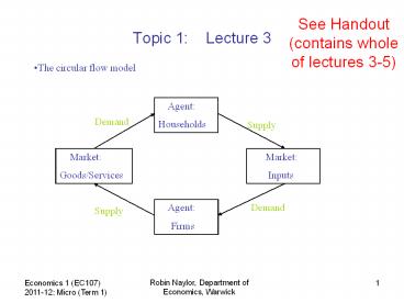
See Handout (contains whole of lectures 3-5) Topic 1: Lecture 3 The circular flow model Agent: Households Demand Supply Market: Goods/Services Market: – PowerPoint PPT presentation
Number of Views:153
Avg rating:3.0/5.0
Title: Topic 1: Lecture 3
1
Topic 1 Lecture 3
See Handout (contains whole of lectures 3-5)
- The circular flow model
Agent Households
Demand
Supply
Market Goods/Services
Market Inputs
Agent Firms
Demand
Supply
2
Topic 1 Lecture 3
- Demand
- Consider a Demand Relation
- What are the influences on Demand for a good . .
. ?
How does a change in some other influence affect
the demand curve?
px
a
po
What does the slope of the demand curve tell us?
b
D
X
Xo
3
Topic 1 Lecture 3
4
Topic 1 Lecture 3
5
Topic 1 Lecture 3
6
Topic 1 Lecture 3
- Supply
- Consider a Supply Relation
- What are the influences on Supply a good . . . ?
How does a change in some other influence affect
the Supply curve?
px
S
What does the slope of the Supply curve tell us?
a
po
b
X
Xo
7
Topic 1 Lecture 3
8
Topic 1 Lecture 3
- Putting together Supply and Demand
What is meant by the market equilibrium?
px
S
What are the possible properties of a market
equilibrium?
pe
D
X
Xe
9
Topic 1 Lecture 3
- Comparative Statics
What is the effect on market equilibrium of a
shift in demand?
px
S
pe
D
X
Xe
10
Topic 1 Lecture 3
- Comparative Statics
What is the effect on market equilibrium of a
shift in supply?
px
S
pe
D
X
Xe
11
Topic 1 Lecture 3
- Uniqueness of equilibrium and price bubbles
Suppose D is the Willingness to Pay for housing.
Its likely to depend on Consumer Confidence
(CC). (i) What happens if CC rises? (ii) What
might cause CC to rise? What is the implication
of this?
px
S
pe
D
X
Xe
12
Topic 1 Lecture 3
13
Topic 1 Lecture 3
14
Topic 1 Lecture 3
15
Topic 1 Lecture 3
16
Topic 1 Lecture 4
Demand Analysis (or analysis of Consumer
Choice) Choice is based on . . . . . .
Preferences and . . . Constraints Well
analyse each of these in turn.
17
Topic 1 Lecture 4
Demand Analysis Preferences Suppose your
happiness depends on just 2 commodities (that
you might buy in the market) e.g., ???
18
Topic 1 Lecture 4
- Demand Analysis Preferences
- E.g., Books and Food
- We assume that you have preferences over these
goods and that the nature of your preferences
satisfies various properties - Non-satiation . . . . . . in words
- Ordinal Ranking
- Transitivity
- Completeness
19
Topic 1 Lecture 4
Demand Analysis Preferences Non-satiation .
. . in a diagram.
B
a
b
B1
F
F1
F2
20
Topic 1 Lecture 4
Demand Analysis Preferences Our assumptions
about the properties of preferences imply that we
can represent preferences using Indifference
Curves. These ICs will have properties which
depend upon the properties of the underlying
preferences.
B
We can show that an IC must slope downwards
because of non-satiation.
a
b
B1
F
F1
F2
21
Topic 1 Lecture 4
Demand Analysis Preferences We can show that
ICs cannot cross under the assumptions we have
made about preferences
IC1
B
IC2
a
c
b
F
22
Topic 1 Lecture 4
Demand Analysis Preferences The slope of the
IC is the MRS between the 2 goods (refer to
earlier slides).
B
a
b
IC1
F
23
Topic 1 Lecture 4
Demand Analysis Preferences If the IC is
linear, this means that the MRS is constant.
B
a
b
IC1
F
24
Topic 1 Lecture 4
Demand Analysis Preferences It is more common
to assume that the MRS is diminishing why is
this and what does it imply about the IC?
B
a
b
F
25
Topic 1 Lecture 4
Demand Analysis Preferences It is more common
to assume that the MRS is diminishing why is
this and what does it imply about the IC?
B
IC1
F
26
Topic 1 Lecture 4
Demand Analysis Preferences What would it
mean if the IC was upward-sloping?
B
IC1
F
27
Topic 1 Lecture 4
Demand Analysis Preferences What would this
mean?
B
IC1
F
28
Topic 1 Lecture 4
Demand Analysis Preferences Under the
assumption of completeness, there is an IC
passing through every possible point
B
b
a
IC2
IC1
F
29
Topic 1 Lecture 4
Demand Analysis Preferences The consumer
would like to get to the highest possible IC
what limits this?
c
ICn
B
b
a
IC2
IC1
F
30
Topic 1 Lecture 5
Demand Analysis Constraints We said that our
understanding of Consumer Choice rests on the
analysis of Preferences and Constraints. Lets
now turn to consider Constraints.
Y
Ymax
X
0
Xmax
31
Topic 1 Lecture 5
Demand Analysis Constraints We can represent
a budget set and a budget frontier (or
constraint)
Y
Ymax
X
0
Xmax
32
Topic 1 Lecture 5
Demand Analysis Constraints We can represent
a budget set and a budget frontier (or
constraint)
Y
What equation can we give this constraint?
Ymax
X
0
Xmax
33
Topic 1 Lecture 5
Demand Analysis Constraints The equation
tells us that if we spend all our money income,
M, on X and Y, our spending be equal to
34
Topic 1 Lecture 5
Demand Analysis Constraints Re-arranging,
the equation for the budget constraint
is How do you interpret this equation? And
Graphically?
35
Topic 1 Lecture 5
Demand Analysis Constraints The equation of
the budget constraint
Y
Ymax
X
0
Xmax
36
Topic 1 Lecture 5
Demand Analysis Constraints Given the
position of the budget constraint, what will be
the consumers choice of X and Y? This will
depend on their preferences
Y
Ymax
X
0
Xmax
37
Topic 1 Lecture 5
Demand Analysis Constrained choice Given the
position of the budget constraint, what will be
the consumers choice of X and Y? This will
depend on their preferences
IC3
Y
IC1
IC2
Ymax
X
0
Xmax
38
Topic 1 Lecture 5
Demand Analysis Constrained choice Given the
position of the budget constraint, what will be
the consumers choice of X and Y? This will
depend on their preferences
ICmax
Y
Ymax
X
0
Xmax
39
Topic 1 Lecture 5
Demand Analysis Constrained choice Given the
position of the budget constraint, what will be
the consumers choice of X and Y? This will
depend on their preferences
Y
Ymax
a
Y
X
0
X
Xmax
40
Topic 1 Lecture 5
Demand Analysis Constrained choice So, by
bringing together preferences and constraints, we
have a model which predicts/explains the
consumers choices (demands) for X and Y . . .
given . . .?
Y
Ymax
a
Y
X
0
X
Xmax
41
Topic 1 Lecture 5
Demand Analysis Comparative Statics What will
happen to the optimal choices of X and Y if there
are relevant changes to the parameters of the
model?
Y
What are the relevant parameters?
Ymax
a
Y
X
0
X
Xmax
42
Topic 1 Lecture 5
Demand Analysis Comparative Statics What will
happen to the optimal choices of X and Y if there
are relevant changes to the parameters of the
model?
Y
Consider a change in money income. How do we show
this?
Ymax
a
Y
X
0
X
Xmax
43
Topic 1 Lecture 5
Demand Analysis Change in money income
Y
Ymax
a
Y
X
0
X
Xmax
44
Topic 1 Lecture 5
Demand Analysis Change in money income
Y
What can you say about the demand for X as
M?? And the demand for Y?
Ymax
â
a
Y
X
0
X
Xmax
45
Topic 1 Lecture 5
Demand Analysis Change in money income
Y
What can you say about the demand for X as
M?? And the demand for Y?
â
Ymax
a
Y
X
0
X
Xmax
46
Topic 1 Lecture 5
Demand Analysis Change in money income
Y
What can you say about the demand for X as
M?? And the demand for Y?
â
Ymax
a
Y
X
0
X
Xmax
47
Topic 1 Lecture 5
Demand Analysis Change in money income
Y
What can you say about the demand for X as
M?? And the demand for Y?
Ymax
â
a
Y
X
0
X
Xmax
48
Topic 1 Lecture 5
Demand Analysis Change in money income
Y
What can you say about the demand for X as
M?? And the demand for Y?
Ymax
a
Y
â
X
0
X
Xmax
49
Topic 1 Lecture 6
See Handout
Demand Analysis Change in price of X
Y
Ymax
What can you say about the demand for X as Px??
Y
a
X
0
X
Xmax
50
Topic 1 Lecture 6
Demand Analysis Change in price of X (CASE 1)
IC1
IC2
Y
Ymax
What can you say about the demand for X as Px??
â
Y
a
X
0
X
Xmax
51
Topic 1 Lecture 6
Demand Analysis Change in price of X (CASE 1)
What is the implication for the shape of the
demand curve for X in (Px, X)space? What is
held constant along this demand curve?
IC1
IC2
Y
Ymax
â
Y
a
X
0
X
Xmax
52
Topic 1 Lecture 6
See Handout
Demand Analysis Change in price of X (CASE 2)
What is the implication for the shape of the
demand curve for X in (Px, X)space? What is
held constant along this demand curve?
IC1
Y
Ymax
IC2
Y
a
â
X
0
X
Xmax
53
Topic 1 Lecture 6
Demand Analysis Change in price of X (CASE 2)
IC1
Y
Ymax
What is the relationship between the price of X,
its demand, and the demand for Y?
IC2
Y
a
â
X
0
X
Xmax
54
Topic 1 Lecture 6
See Handout
Demand Analysis Change in price of X (CASE 3)
IC1
Y
IC2
Ymax
What is the implication for the shape of the
demand curve for X in (Px, X)space?
â
Y
a
X
0
X
Xmax
55
Topic 1 Lecture 6
Demand Analysis Change in price of X (CASE 3)
IC1
Y
IC2
Ymax
What is the relationship between the price of X,
its demand, and the demand for Y?
â
Y
a
X
0
X
Xmax
56
Topic 1 Lecture 6
See Handout
Demand Analysis Change in price of X (CASE 4)
IC1
IC2
Y
Ymax
What is the implication for the shape of the
demand curve for X in (Px, X)space?
â
Y
a
X
0
X
Xmax
57
Topic 1 Lecture 6
See Handout
Demand Analysis Change in price of X (CASE 3
Revisited)
- There are 2 reasons for the rise in demand for X
following the fall in its price - Disposable (or real) Income Effect
- Relative Price Effect
Y
Ymax
â
Y
a
X
0
X
Xmax
58
Topic 1 Lecture 6
See Handout
Demand Analysis Change in price of X (CASE 3
Revisited)
- There are 2 reasons for the rise in demand for X
following the fall in its price - Disposable (or real) Income Effect
- The budget constraint shifts outwards and hence
the individual can achieve higher utility that
is, move on to previously unobtainable
Indifference Curves. They are able to buy more of
both X and Y whether or not they do so will
depend on their preferences over X and Y. If X is
normal, for example, the Real Income Effect will
cause the individual to buy more X. - Relative Price Effect
- X is now relatively cheaper than previously
relative to Y. The individual is therefore likely
to switch from Y towards X, to some extent.
59
Topic 1 Lecture 6
See Handout
Demand Analysis Change in price of X (CASE 3
Revisited)
- We would now like to be able to distinguish
between these two effects in the diagram. - Real Income Effect
- Relative Price Effect
Y
Ymax
â
Y
a
X
0
X
Xmax
60
Topic 1 Lecture 6
Demand Analysis Change in price of X (CASE 3
Revisited)
Consider first the Relative Price
Effect. Suppose relative prices had changed, but
that there had been no Real Income Effect of the
price change. What point in the diagram could
represent such a position?
Y
Ymax
â
Y
a
X
0
X
Xmax
61
Topic 1 Lecture 6
Demand Analysis Change in price of X (CASE 3
Revisited)
Consider first the Relative Price
Effect. Suppose relative prices had changed, but
that there had been no Real Income Effect of the
price change. What point in the diagram could
represent such a position? b
Y
Ymax
â
Y
a
b
X
0
X
Xmax
62
Topic 1 Lecture 6
Demand Analysis Change in price of X (CASE 3
Revisited)
Relative Price Effect. What change is causing
the consumer equilibrium to move from a to
b? What is not changing between a and
b? Hence, a to b represents a pure
relative price effect.
Y
Ymax
â
Y
a
b
As a and b lie on the same IC, there is no
Real Income change in moving from a to b.
X
0
X
Xmax
63
Topic 1 Lecture 6
Demand Analysis Change in price of X (CASE 3
Revisited)
Relative Price Effect. a to b represents a
pure relative price effect. More commonly, we
refer to it as a substitution effect
Y
Ymax
â
Y
a
b
S
X
0
X
Xs
Xmax
64
Topic 1 Lecture 6
Demand Analysis Change in price of X (CASE 3
Revisited)
Real Income Effect. We claimed that the Total
Effect of the price change (i.e., from a to
â) is made up of a Relative Price
(Substitution) Effect and a Real Income Effect.
Y
Ymax
â
Y
a
b
As a to b is the substitution effect, can we
show that b to â is the Real Income Effect?
S
X
0
X
Xs
Xmax
65
Topic 1 Lecture 6
Demand Analysis Change in price of X (CASE 3
Revisited)
Real Income Effect. Compare b and â. What
have they got in common? What is different
between them? Your answers should confirm for you
that b to â captures the Real Income Effect.
Y
Ymax
â
Y
a
b
As a to b is the substitution effect, can we
show that b to â is the Real Income Effect?
S
I
X
0
X
Xs
X
66
Topic 1Lecture 7
See Handout
Px
Deriving demand curves
The total effect of the price change is to move
the consumers choice from a to â.
a
â
b
X
Px
a
If we plot this into the lower diagram, what are
we plotting?
X
67
Topic 1Lecture 7
Px
The total effect of the price change is to move
the consumers choice from a to â.
a
â
b
X
Px
a
If we plot this into the lower diagram, what are
we plotting?
â
X
68
Topic 1Lecture 7
Px
The total effect of the price change is to move
the consumers choice from a to â.
a
â
b
X
Px
a
If we plot this into the lower diagram, what are
we plotting?
â
?
X
69
Topic 1Lecture 7
Px
The total effect of the price change is to move
the consumers choice from a to â.
a
â
b
X
Px
a
If we plot this into the lower diagram, what are
we plotting?
What can you say about the slope of this curve?
Must it be ve?
â
CMIDC
X
70
Topic 1Lecture 7
Px
The Substitution Effect of the price change is to
move the consumers choice from a to b.
a
â
b
S
X
Px
a
If we plot this into the lower diagram, what are
we plotting?
b
S
?
X
71
Topic 1Lecture 7
Px
The Substitution Effect of the price change is to
move the consumers choice from a to b.
a
â
b
S
X
Px
a
If we plot this into the lower diagram, what are
we plotting?
b
S
CUDC/CRIDC
X
72
Topic 1Lecture 7
Px
The Substitution Effect of the price change is to
move the consumers choice from a to b.
a
â
b
S
X
Px
a
b
Must this curve have a ve slope?
S
CUDC/CRIDC
X
73
Topic 1Lecture 7
The Substitution Effect of the price change is to
move the consumers choice from a to b.
Px
The Income Effect of the price change is to move
the consumers choice from b to â.
a
â
b
S
I
X
The Substitution Effect determines the CRIDC.
The Substitution Effect combined with the Income
Effect determines the CMIDC.
Px
a
b
S
I
CRIDC
X
74
Topic 1Lecture 7
The Substitution Effect of the price change is to
move the consumers choice from a to b.
Px
The Income Effect of the price change is to move
the consumers choice from b to â.
a
â
b
S
I
X
The Substitution Effect determines the CRIDC.
The Substitution Effect combined with the Income
Effect determines the CMIDC.
Px
a
b
â
CMIDC
S
I
CRIDC
X
75
Topic 1Lecture 7
The Substitution Effect of the price change is to
move the consumers choice from a to b.
See Handout
Px
The Income Effect of the price change is to move
the consumers choice from b to â.
The difference between the CRIDC and the CMIDC is
the Income Effect. In this diagram, X is a
Normal Good. Therefore, the CMIDC is more
elastic than the CRIDC
a
â
b
S
I
X
The Substitution Effect determines the CRIDC.
The Substitution Effect combined with the Income
Effect determines the CMIDC.
Px
a
b
â
CMIDC
S
I
CRIDC
X
76
Topic 1Lecture 7
The Substitution Effect of the price change is to
move the consumers choice from a to b.
See Handout
Px
The difference between the CRIDC and the CMIDC is
the Income Effect. In this diagram, X is a
Weakly Inferior Good. Therefore, the CMIDC is
less elastic than the CRIDC
â
The Income Effect of the price change is to move
the consumers choice from b to â.
a
b
S
I
X
The Substitution Effect determines the CRIDC.
The Substitution Effect combined with the Income
Effect determines the CMIDC.
Px
a
b
â
S
I
CRIDC
CMIDC
X
77
Topic 1Lecture 7
The Substitution Effect of the price change is to
move the consumers choice from a to b.
See Handout
Px
â
The difference between the CRIDC and the CMIDC is
the Income Effect. In this diagram, X is a
Strongly Inferior Good. Therefore, the CMIDC is
vely sloped.
The Income Effect of the price change is to move
the consumers choice from b to â.
a
b
I
S
X
The Substitution Effect determines the CRIDC.
The Substitution Effect combined with the Income
Effect determines the CMIDC.
Px
a
b
â
CMIDC ?
I
S
CRIDC
X
78
Topic 1Lecture 7
The Substitution Effect of the price change is to
move the consumers choice from a to b.
Px
â
The difference between the CRIDC and the CMIDC is
the Income Effect. In this diagram, X is a
Strongly Inferior Good. Therefore, the CMIDC is
vely sloped. (Giffen Good)
The Income Effect of the price change is to move
the consumers choice from b to â.
a
b
I
S
X
The Substitution Effect determines the CRIDC.
The Substitution Effect combined with the Income
Effect determines the CMIDC.
Px
a
b
â
I
S
CMIDC
CRIDC
X
79
Topic 1 Lecture 8
See Handout
Market Demand
p
p
p
?
D2
D1
X
01
02
0M
80
Topic 1 Lecture 8
Market Demand
p
p
p
D2
D1
X
01
02
0M
81
Topic 1 Lecture 8
Market Demand Horizontal Summation
(Why?) (Note well see a case of vertical
summation later in the module) Notice than in
the 2-person case above, the market demand curve
is kinked.
p
p
p
DM
D2
D1
X
01
02
0M
82
Topic 1 Lecture 8
See Handout
Consumer Surplus Interpret the
Marginal Willingness to Pay (Marginal Benefit,
Marginal Valuation)
p
S
p
D
X
0
X
83
Topic 1 Lecture 8
Consumer Surplus Consumer Surplus on
first unit.
p
S
p
D
X
0
X
84
Topic 1 Lecture 8
Consumer Surplus Consumer Surplus on
all units.
p
S
A
p
D
0
X
85
Topic 1 Lecture 8
See Handout
Demand Elasticity We have already said that the
Price Elasticity of Demand for a Good is a
measure of the sensitivity or responsiveness of
demand for a good to a change in its price. More
precisely
86
Topic 1 Lecture 8
See Handout
Demand Elasticity
87
Topic 1 Lecture 8
See Handout
Demand Elasticity
88
Topic 1 Lecture 8
See Handout
Demand Elasticity
0
-1
89
Topic 1 Lecture 8
See Handout
Demand Elasticity
0
-1
90
Topic 1 Lecture 9
See Handout
Importance of Elasticity Suppose the
Government raises the indirect tax on this
commodity. How do we show this?
p
S
p
D
X
0
X
91
Topic 1 Lecture 9
ST
Importance of Elasticity What is the
Tax Revenue . . . ?
p
S
p
D
X
0
X
92
Topic 1 Lecture 9
ST
Importance of Elasticity What is the
Tax Revenue? What is the Tax Burden?
p
S
A
p
B
D
X
0
X
93
Topic 1 Lecture 9
ST
Importance of Elasticity What is
the Tax Burden? How would the shares of the tax
burden change with a different price elasticity
of demand for the good?
ST
p
p
S
S
A
p
B
D
X
0
X
0
X
94
Topic 1 Lecture 9
ST
Importance of Elasticity What is
the Tax Burden? How would the shares of the tax
burden change with a different price elasticity
of demand for the good?
ST
p
p
S
S
A
p
B
D
D
X
0
X
0
X
95
Topic 1 Lecture 9
ST
Importance of Elasticity How would
the shares of the tax burden change with a
different price elasticity of demand for the
good? Why is this?
ST
p
p
S
S
A
A
p
B
B
D
D
X
0
X
0
X
96
Topic 1 Lecture 10
See Handout
Applications of Consumer Choice Theory 1. Labour
Supply The Income-Leisure Trade-off
Income
IC
Leisure
97
Topic 1 Lecture 10
Labour Supply The Income-Leisure Trade-off
Tmax
Income
Time Constraint Tmax
IC
Tmax
0
Leisure
Labour Supply
0
98
Topic 1 Lecture 10
Labour Supply The Income-Leisure Trade-off
Tmax
Income
Wage Constraint w (wage per hour)
w
Tmax
0
Leisure
Labour Supply
0
99
Topic 1 Lecture 10
Labour Supply The Income-Leisure Trade-off
Tmax
Income
Wage Constraint w (wage per hour) And Non-labour
income, N.
w
N
Tmax
0
Leisure
Labour Supply
0
100
Topic 1 Lecture 10
Labour Supply The Income-Leisure Trade-off
Tmax
Optimisation, given w, N and Tastes. Total
Income Labour Income Non-Labour
Income Total Income Y N
Income
Y
IC
w
N
N
Tmax
0
L
Leisure
Labour Supply
0
101
Topic 1 Lecture 10
Labour Supply The Income-Leisure Trade-off
Tmax
Optimisation, given w, N and Tastes. What
happens to optimal Labour Supply if N rises (why
might it?)?
Income
Y
IC
w
N
N
Tmax
0
L
Leisure
Labour Supply
0
102
Topic 1 Lecture 10
See Handout
Labour Supply The Income-Leisure Trade-off
Tmax
What happens to optimal Labour Supply if N rises
Income
IC
N
Tmax
0
Leisure
103
Topic 1 Lecture 10
Labour Supply The Income-Leisure
Trade-off
Tmax
What happens to optimal Labour Supply if N
rises? Under what assumption? Why?
Income
b
IC
a
IC
N
Tmax
0
Leisure
104
Topic 1 Lecture 10
See Handout
Labour Supply The Income-Leisure Trade-off
Tmax
Income
w
a
a
w
Y
IC
w
N
N
L, Labour Supply
L
Tmax
0
L
Leisure
Labour Supply
0
What happens to optimal Labour Supply if w rises?
105
Topic 1 Lecture 10
Tmax
Income
w
a
a
IC
w
N
L, Labour Supply
L
Tmax
0
L
Leisure
Labour Supply
0
What happens to optimal Labour Supply if w rises?
106
Topic 1 Lecture 10
Tmax
Income
w
a
a
a
IC
w
L, Labour Supply
L
Tmax
0
L
Leisure
Labour Supply
0
What happens to optimal Labour Supply if w rises?
107
Topic 1 Lecture 10
Tmax
Income
w
a
a
a
a
IC
L, Labour Supply
L
Tmax
0
L
Leisure
Labour Supply
0
What is the implied shape of the Labour Supply
curve in this case?
108
Topic 1 Lecture 10
Tmax
Income
w
a
Ls
a
IC
L, Labour Supply
L
Tmax
0
L
Leisure
Labour Supply
What is the implied shape of the Labour Supply
curve in this case? And the elasticity of Labour
Supply?
0
109
Topic 1 Lecture 10
See Handout
To understand how labour supply responds to a
change in the wage rate, it is useful to exploit
the distinction between Income and Substitution
Effects. To do this, we need to shift back the
new Budget Line until it is just a tangent to the
original Indifference Curve . . .
Tmax
Income
a
a
IC
Tmax
0
L
Leisure
Labour Supply
0
110
Topic 1 Lecture 10
To understand how labour supply responds to a
change in the wage rate, it is useful to exploit
the distinction between Income and Substitution
Effects. To do this, we need to shift back the
new Budget Line until it is just a tangent to the
original Indifference Curve . . .
Tmax
Income
a
a
Tmax
0
L
Leisure
Labour Supply
0
111
Topic 1 Lecture 10
To understand how labour supply responds to a
change in the wage rate, it is useful to exploit
the distinction between Income and Substitution
Effects. To do this, we need to shift back the
new Budget Line until it is just a tangent to the
original Indifference Curve . . . with the move
from a to a split into a gt b
Substitution Effect, b gt a Income
Effect.
Tmax
Income
a
b
a
I
S
Tmax
0
L
Leisure
Labour Supply
0
112
Topic 1 Lecture 10
Tmax
Income
a gt b Substitution Effect, b gt
a Income Effect. When the Substitution and
Income Effects just cancel each other out, the
rise in the wage rate has no net effect on Labour
Supply and the derived Labour Supply curve is
vertical, as we have seen.
a
b
a
I
S
Tmax
0
L
Leisure
Labour Supply
0
113
Topic 1 Lecture 10
a gt b Substitution Effect, b gt
a Income Effect. How would you interpret
the Income Effect in words? And the Substitution
Effect (Hint exploit the concept of the
Opportunity Cost)
Tmax
Income
a
b
a
I
S
Tmax
0
L
Leisure
Labour Supply
0
114
Topic 1 Lecture 10
a gt b Substitution Effect, b gt
a Income Effect. When the Substitution and
Income Effects just cancel each other out, the
rise in the wage rate has no net effect on Labour
Supply and the derived Labour Supply curve is
vertical, as we have seen. What about if the
Substitution Effect dominates? What is the shape
of the Labour Supply curve in this case?
Tmax
Income
a
b
a
I
S
Tmax
0
L
Leisure
Labour Supply
0
115
Topic 1 Lecture 10
When the S-effect dominates the I-effect
Tmax
Income
w
a
a
Ls
a
a
I
S
L, Labour Supply
L
Tmax
0
L
Leisure
Labour Supply
What is the implied shape of the Labour Supply
curve in this case? And the elasticity of Labour
Supply?
0
116
Topic 1 Lecture 10
See Handout
When the S-effect dominates the I-effect
Tmax
Income
w
Ls
a
a
a
a
I
S
L, Labour Supply
L
Tmax
0
L
Leisure
Labour Supply
What is the implied shape of the Labour Supply
curve in this case? And the elasticity of Labour
Supply?
0
117
Topic 1 Lecture 10
See Handout
When the I-effect dominates the S-effect
Tmax
Income
w
Ls
a
a
a
a
I
S
L, Labour Supply
L
Tmax
0
L
Leisure
Labour Supply
What is the implied shape of the Labour Supply
curve in this case? And the elasticity of Labour
Supply?
0
118
Topic 1 Lecture 10
See Handout
Labour Supply the evidence . .
. And for most people? And the
implication for income tax cuts?
Ls
w
L
119
Topic 1 Lecture 11
See Handout
Applications of Consumer Choice
Theory 2. Inter-temporal Choice
Think of an Endowment Point and add it to the
diagram.
I1 , C1
I0 , C0
120
Topic 1 Lecture 11
Inter-temporal Choice
From the Endowment Point, where can Saving take
you? And Borrowing?
I1 , C1
E
I1
I0 , C0
I0
121
Topic 1 Lecture 11
Inter-temporal Choice
From the Endowment Point, where can Saving take
you? (And Borrowing?)
I1 , C1
E
I1
I0 , C0
I0
122
Topic 1 Lecture 11
Inter-temporal Choice
From the Endowment Point, where can Saving take
you? (And Borrowing?)
I1 , C1
1i
E
I1
1
I0 , C0
I0
One Euro saved this period yields one Euro plus
(one Euro times the rate of interest) next
period. Or . . .
123
Topic 1 Lecture 11
Inter-temporal Choice
From the Endowment Point, where can Saving take
you?
I1 , C1
E
I1
I0 , C0
I0
Or . . .
124
Topic 1 Lecture 11
Inter-temporal Choice
From the Endowment Point, where can Saving take
you?
I1 , C1
C1
E
I1
I0 , C0
I0
C0
Or . . .
125
Topic 1 Lecture 11
Inter-temporal Choice
From the Endowment Point, where can Saving take
you? What is the slope of the budget
constraint?
I1 , C1
C1
E
I1
I0 , C0
I0
C0
Or . . .
126
Topic 1 Lecture 11
See Handout
Inter-temporal Choice
From the Endowment Point, where can Borrowing
take you?
I1 , C1
E
I1
C1
I0 , C0
I0
C0
Or . . .
127
Topic 1 Lecture 11
Inter-temporal Choice
From the Endowment Point, where can all possible
Saving or Borrowing take you? This is the
inter-temporal budget constraint.
I1 , C1
E
I1
I0 , C0
I0
128
Topic 1 Lecture 11
See Handout
Inter-temporal Choice
I1 , C1
What is the value of C1? (Note the value of the
slope.)
C1
E
I1
I0 , C0
I0
C0
129
Topic 1 Lecture 11
Inter-temporal Choice
I1 , C1
Re-arranging
C1
E
I1
I0 , C0
I0
C0
130
Topic 1 Lecture 11
Inter-temporal Choice
I1 , C1
C1
E
I1
This is the horizontal intercept of the budget
constraint. What is its interpretation?
I0 , C0
I0
C0
131
Topic 1 Lecture 11
See Handout
Inter-temporal Choice
How would you show the effect on the
inter-temporal budget constraint of a fall in the
rate of interest?
I1 , C1
C1
E
I1
I0 , C0
I0
C0
132
Topic 1 Lecture 11
Inter-temporal Choice
What happens to the Present Value of E after a
fall in the rate of interest?
I1 , C1
C1
E
I1
I0 , C0
I0
C0
133
Topic 1 Lecture 11
See Handout
Inter-temporal Choice
How would you represent an individuals
preferences over consumption today and tomorrow?
I1 , C1
E
I1
I0 , C0
I0
134
Topic 1 Lecture 11
Inter-temporal Choice
What does the slope of the indifference curve
represent? If the MRTP is high (low), what does
this mean?
I1 , C1
E
I1
I0 , C0
I0
135
Topic 1 Lecture 11
See Handout
Inter-temporal Choice
I1 , C1
Optimisation.
I1
E
A
C1
I0 , C0
I0
C0
136
Topic 1 Lecture 11
Inter-temporal Choice
I1 , C1
Is this person saving or borrowing?
I1
E
A
C1
I0 , C0
I0
C0
137
Topic 1 Lecture 11
Inter-temporal Choice
I1 , C1
How will they respond to a fall in the rate of
interest?
I1
E
A
C1
I0 , C0
I0
C0
138
Topic 1 Lecture 11
See Handout
Inter-temporal Choice
I1 , C1
How will they respond to a fall in the rate of
interest? Consider the substitution effect.
I1
E
A
C1
I0 , C0
I0
C0
139
Topic 1 Lecture 11
Inter-temporal Choice
Borrowing is cheaper and so the borrower borrows
more (Substitution effect). They are also better
off (why?) so there is an Income effect. Which
way does Income effect go?
I1 , C1
I1
E
A
C1
I0 , C0
I0
C0
140
Topic 1 Lecture 11
Inter-temporal Choice
Borrowing is cheaper and so the borrower borrows
more (Substitution effect). They are also better
off (why?) so there is an Income effect. Which
way does Income effect go?
I1 , C1
I1
E
A
C1
B
I0 , C0
I0
C0
S
I
141
Topic 1 Lecture 11
Inter-temporal Choice
So fall in the rate of interest leads Borrower to
borrow more unless Consumption today is a . . .
. ? Good.
I1 , C1
I1
E
A
C1
B
I0 , C0
I0
C0
S
I
142
Topic 1 Lecture 11
See Handout
Inter-temporal Choice
How would you show the effect on a Borrower of a
rise in the interest rate? Will the Borrower
borrow more or less? On what does your answer
depend?
I1 , C1
I1
E
A
C1
I0 , C0
I0
C0
143
Topic 1 Lecture 11
See Handout
Inter-temporal Choice
How would you show the effect on a Saver of a
rise in the interest rate? Will the Saver save
more or less? On what does your answer depend?
I1 , C1
A
C1
E
I1
I0 , C0
I0
C0
144
Topic 1 Lecture 11
See Handout
Inter-temporal Choice
How would you show the effect on a Saver of a
fall in the interest rate? Will the Saver save
more or less? On what does your answer depend?
I1 , C1
A
C1
E
I1
I0 , C0
I0
C0
145
Topic 1 Lecture 11
See Handout
Intertemporal Choice
146
Topic 1 Lecture 12
See Handout
Gains from Trade Consider an industry in an
Autarkic country
p
What is the extent of Consumer Surplus in this
case?
Sd
pd
Dd
X
Xd
147
Topic 1 Lecture 12
Gains from Trade Consider an industry in an
Autarkic country
p
What is the extent of Consumer Surplus in this
case?
Sd
A
pd
Dd
X
Xd
148
Topic 1 Lecture 12
Gains from Trade Consider an industry in an
Autarkic country
p
And Producer Surplus in this case?
Sd
A
pd
Dd
X
Xd
149
Topic 1 Lecture 12
Gains from Trade Consider an industry in an
Autarkic country
p
And Producer Surplus in this case?
Sd
A
pd
B
Dd
X
Xd
150
Topic 1 Lecture 12
See Handout
Gains from Trade Consider an industry in an
Autarkic country
p
Suppose that in the Rest of the World, the World
Price of X, pw, was higher than pd. What would
this mean?
Sd
pw
pw
pd
Dd
X
Xd
151
Topic 1 Lecture 12
Gains from Trade Consider trade. Suppose the
World Price exceeds the Domestic Autarkic price
p
Sd
Domestic Firms would not be prepared to sell any
units at the low price of pd. They will sell at
the World Price by exporting to the Rest of the
World at the World Price of pw. Domestic Demand
(and sales) are equal to Xdt at the world price.
pw
pw
pd
Dd
X
Xd
Xdt
152
Topic 1 Lecture 12
Gains from Trade Consider trade. Suppose the
World Price exceeds the Domestic Autarkic price
p
Sd
Domestic Firms would not be prepared to sell any
units at the low price of pd. They will sell at
the World Price by exporting to the Rest of the
World at the World Price of pw. Effectively,
the Domestic Firms Supply curve becomes the one
in bold. Be sure you can explain this to yourself.
pw
pw
pd
Dd
X
Xd
Xdt
153
Topic 1 Lecture 12
Gains from Trade Consider trade. Suppose the
World Price exceeds the Domestic Autarkic price
p
Sd
Effectively, the Domestic Firms Supply curve
becomes the one in bold. Be sure you can explain
this to yourself. Total Domestic Firm sales are
given by Xt. Exports are equal to Xt Xdt.
pw
pw
pd
Dd
X
Xd
Xdt
Xt
154
Topic 1 Lecture 12
See Handout
Gains from Trade Consider trade. Suppose the
World Price exceeds the Domestic Autarkic price
p
Sd
What has happened to CS and PS, and hence total
welfare, in this country under the equilibrium
with trade compared to the total welfare (CSPS)
in this country under Autarky? So Who Gains and
Who Loses from Trade (and by how much in each
case)? Work it out for yourself.
pw
pw
pd
Dd
X
Xd
Xdt
Xt
155
Topic 1 Lecture 12
See Handout
Gains from Trade Consider an industry in an
Autarkic country
p
Suppose that in the Rest of the World, the World
Price of X, pw, was lower than pd. What would
this mean?
Sd
pd
pw
pw
Dd
X
Xd
156
Topic 1 Lecture 12
Gains from Trade Consider trade. Suppose the
World Price is less than the Domestic Autarkic
price
p
Domestic buyers would not be prepared to buy any
units at the high price of pd. They will want to
buy at the World Price by importing from the Rest
of the World at the World Price of pw. Domestic
Supply (and hence sales) are equal to Xdt at the
world price.
Sd
pd
pw
pw
Dd
X
Xd
Xdt
157
Topic 1 Lecture 12
Gains from Trade Consider trade. Suppose the
World Price is less than the Domestic Autarkic
price
p
Domestic buyers would not be prepared to buy any
units at the high price of pd. Effectively, the
Domestic Buyers Demand curve becomes the one in
bold. Be sure you can explain this to yourself.
Sd
pd
pw
pw
Dd
X
Xd
Xdt
158
Topic 1 Lecture 12
Gains from Trade Consider trade. Suppose the
World Price is less than the Domestic Autarkic
price
p
Effectively, the Domestic Buyers Demand curve
becomes the one in bold. Be sure you can explain
this to yourself. Total Domestic Buyers
consumption is given by Xt. Imports are equal to
Xt Xdt.
Sd
pd
pw
pw
Dd
X
Xd
Xdt
Xt
159
Topic 1 Lecture 12
See Handout
Gains from Trade Consider trade. Suppose the
World Price is less than the Domestic Autarkic
price
p
What has happened to CS and PS, and hence total
welfare, in this country under the equilibrium
with trade compared to the total welfare (CSPS)
in this country under Autarky? So Who Gains and
Who Loses from Trade (and by how much in each
case)? Work it out for yourself.
Sd
pd
pw
pw
Dd
X
Xd
Xdt
Xt
160
Topic 1 Lecture 12
See Handout
Gains from Trade Consider trade. Suppose the
World Price is less than the Domestic Autarkic
price
p
In the case of a country where there are imports,
there might be calls for tariffs or import
quotas. What would be the welfare effects of
each of these? What factors influence the
magnitudes of the effects?
Sd
pd
pw
pw
Dd
X
Xd
Xdt
Xt
161
Topic 1
See Handout
- Key Concepts
- The circular flow model
- A simple model of a market
- Consumer choice basic setup
- Preferences, indifference curves and utility
- Budget constraints
- Consumer equilibrium utility maximization
- The algebra of consumer equilibrium
- Income consumption curves
- Price consumption and the derived demand curves
162
Topic 1
See Handout
- Key Concepts
- The algebra of deriving the demand curve
- The compensated demand curve
- Income and substitution effects of a price change
- Normal, inferior and Giffen goods
- Consumer surplus
- Market demand
- The price elasticity of demand
- Tax incidence
- Winners and Losers from Trade
- Labour supply by the household
- Capital supply by the household
163
Topic 1
See Handout
- Key Readings
- Frank, Chapters 1-5
- Estrin, Laidler and Dietrich, Chapters 1-6
- Online resources
- http//www.bized.ac.uk/current/index.htm
- http//www.bized.ac.uk/learn/economics/index.htm
164
Topic 1
See Handout
- Seminar Questions weeks 4, 6
- (Note Questions in bold (i.e., 1, 2, 6, 8,
11,17) are the questions on which Seminars should
focus. Other questions are preparatory and would
be good self-study questions to address ahead of
seminar meetings) - Explain what economists mean by the term market
equilibrium. - What is meant by the following properties of an
equilibrium - Existence
- Uniqueness
- Stability
- What is likely to happen to the demand curve if
money incomes of consumers rise, ceteris paribus?
(What is meant by ceteris paribus?) - What factors are held constant along the demand
curve? - What factors are held constant along the supply
curve? - Explain the difference between a movement along
the demand curve and a shift of the demand curve.
165
Topic 1
See Handout
- Seminar Questions weeks 4, 6 continued
- What are the comparative static properties of a
typical market equilibrium (for example, what is
likely to happen to the market equilibrium if
there is an increase in consumers money income)? - What are the principal properties of indifference
curves? How do these properties relate to the
assumptions we make regarding the consumers
underlying preferences? - Using indifference curve analysis, show how the
demand for a good responds to a rise in money
income, for each of the following cases - A normal good
- A necessity
- An inferior good
- Using indifference curve analysis, show how the
demand for a good might respond to a change in
the price of that good. - Show how to decompose the effects of a price
change into both income and substitution effects,
for each of the possible cases you have
considered. - Explain intuitively what income and substitution
effects are.
166
Topic 1
See Handout
- Seminar Questions weeks 4, 6 continued
- Why is the market demand curve derived by
horizontal (rather then by vertical) summation of
the individuals demand curves? - Is the market demand curve necessarily kinked
(like in the figure in the lecture notes)? - Define what is meant by Consumer Surplus. How do
you represent Consumer Surplus in a diagram? - Define what is meant by the (own-) price
elasticity of demand for a good. - What happens to the elasticity of demand as we
move along the linear demand curve? - If a proportional tax rate on labour income is
cut, what are the possible implications for the
optimal labour supply choices of workers? Explain
your answer using diagrams and be careful to
distinguish between Income and Substitution
Effects. - If the rate of interest rises, will savers save
more? Will borrowers borrow less? - Further Self-study question suggestions
- Try as many as you can of the discussion
questions at the end of each of the chapters in
Katz and Rosen (or Morgan et al.) and of the
problems at the end of each of the chapters in
Estrin et al..
Recommended
CrystalGraphics Presentations


