Cavendish Experiment

1
Procedure I

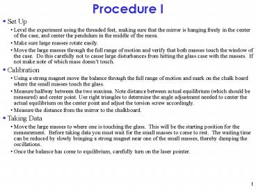
• Set Up
• Level the experiment using the threaded feet,
  making sure that the mirror is hanging freely in
  the center of the case, and center the pendulum
  in the middle of the mesa.
• Make sure large masses rotate easily.
• Move the large masses through the full range of
  motion and verify that both masses touch the
  window of the case. Do this carefully not to
  cause large disturbances from hitting the glass
  case with the masses. If not make note of which
  mass doesnt touch.
• Calibration
• Using a strong magnet move the balance through
  the full range of motion and mark on the chalk
  board where the small masses touch the glass.
• Measure halfway between the two maxima. Note
  distance between actual equilibrium (which should
  be measured) and center point. Use right
  triangles to determine the angle adjustment
  needed to center the actual equilibrium on the
  center point and adjust the torsion screw
  accordingly.
• Measure the distance from the mirror to the
  chalkboard.
• Taking Data
• Move the large masses to where one is touching
  the glass. This will be the starting position
  for the measurement. Before taking data you must
  wait for the small masses to come to rest. The
  waiting time can be reduced by slowly bringing a
  strong magnet near one of the small masses,
  thereby damping the oscillations.
• Once the balance has come to equilibrium,
  carefully turn on the laser pointer.

1
2
Procedure II

• Making measurements
• At t0, after the small masses have stabilized in
  Position I, make a mark to indicate initial
  position and switch the Masses to Position II
• Make marks every 15sec for 45min for each
  position
• Switch to Position I, and repeat the same process
• Marking extrema may improve results
• It may be helpful to write down the time every
  few minutes, to keep track of data when
  calculating
• Calculating Equilibrium positions
• Take two separate averages of all marks for
  positions I and II, making sure there are an
  equal number of maxima in each direction

2
3
Fall 2012 Equilibrium Data

• The measurements resulted in G5.12x10-11
  m3/kg/s223 less than the accepted value
• Given that the experimental error is within 16 ,
  this result is confusing. We do not have an
  explanation for it at this time.

3
4
Fall 2012 Constant Accel. Data

• The measurements from Series 1 resulted in G
  5.23x10-11 m3/kg/s222 less than the accepted
  valueand the measurements from Series 2 resulted
  in G 6.16x10-11 m3/kg/s27.7 less than the
  accepted value.
• Given that the experimental error is 10 and 9,
  respectively, the first result is confusing and
  the second is acceptable. We do not have an
  explanation for this at this time.

4
5
Error Discussion

• There were giant problems with error
• Constant acceleration method had 1951919335
  error
• Equilibrium method had 117983750 to
  138881057 error
• However, there are still errors beyond Pascos
  estimates
• Possible sources of error include
• The mirror is not planar, it is concave.
• If mirror moves laterally, lasers incident angle
  will change.
• If laser is not centered properly on the mirror,
  incident angle will not change linearly with
  mirror rotation.
• Inaccuracies in measuring the equilibrium
  positions on the graphs
• Definitely accounts for some of the error.
• The separation of the large and small balls, b,
  is taken to be constant
• it actually changes throughout the experiment.

5
6
Compare With Coulomb Experiment
A Note on Previous Presentations

• Previous versions of this PowerPoint contained
  the following slide

• Forces are much smaller
• Typical Coulomb force 10-4 N (with V 6kV for
  both spheres, and distance 8cm)
• Typical Cavendish force 10-9 N (with distance
  46.5 mm, m120g, m21.5kg
• Both require a correction factor
• Coulomb experiment requires a correction factor
  of 1/(1-a3/R3)
• a is the radius of the sphere, R is the distance
  between spheres
• This is because the sphere is not a point charge
• Cavendish experiment requires a correction factor
  of 1/(1-b)
• b is the distance between the spheres
• This is because there is gravitational force
  between each small mass and both large masses,
  but only one is considered in the calculations.

• This inserts a correction factor with no
  explanation of its derivation.

7
A Note on Previous Presentations

• Fcorrection G m1 m2 / h2
• h (2d)2 (b sin ?)21/2
• Torquecorrection d x Fcorrection d
  Fcorrection sin ?
• Torquegrav-corrected 2 F d 2 d Fcorrection
  sin ? ?? 2G m1 m2 d / b2 2G m1 m2 d /
  (2d)2 (b sin ?)2
• G ?? / (2 m1 m2 d / b2 2 m1 m2 d / (2d)2
  (b sin ?)2 ? deltaS (4L)-1 (2 m1 m2 d / b2
  2 m1 m2 d / (2d)2 (b sin ?)2)-1 4 pi2 I
  deltaS (4LT2)-1 (2 m1 m2 d / b2 2 m1 m2 d /
  (2d)2 (b sin ?)2)-1 8 pi2 m2 (d2 2/5r2)
  deltaS (4LT2d)-1 (2 m1 m2 / b2 2 m1 m2 /
  (2d)2 (b sin ?)2)-1 pi2 (d2 2/5r2) deltaS
  / (L T2 d m1) / (1/ b2 1 / (2d)2 (b sin
  deltaS / (4L))2)

8
A Note on Previous Presentations

• Using Mathematica to equate the result on the
  previous slide with the result derived earlier,
  the correction factor is (4 d2 b2
  SindeltaS/(4 L)2)/(b2 4 d2 b2
  SindeltaS/(4 L)2)So multiplying the original
  result by this factor gives the corrected result
  for G. Using the values stated earlier, this
  gives a correction factor equal to approximately
  0.83.
• Since this is not negligible, we must include it
  in our final result.

9
Procedure I

• Set Up
• Level the experiment using the threaded feet,
  making sure that the mirror is hanging freely in
  the center of the case , and center the pendulum
  in the middle of the mesa.
• Make sure that when the large masses are moved
  that the small masses only experience small
  oscillations.
• Move the large masses through the full range of
  motion and verify that both masses touch the
  window of the case. Do this carefully not to
  cause large disturbances from hitting the glass
  case with the masses. If not make note of which
  mass doesnt touch.
• Calibration
• Using a strong magnet move the balance through
  the full range of motion and mark on the graph
  paper where the small masses touch the glass.
• To center the natural equilibrium position, we
  would move one small tick mark. Then we would
  watch which direction the masses moved towards
  and would move it another small tick if the
  movement was away from the center. Initially, one
  could move 2 small tick marks if one was not near
  the center already. The angular variation in
  equilibrium points from switching the
  mass-positions was approx. 0.01 rad 0.8º. The
  total angular variation from maximums was 2.5º.
• Measure the distance from the mirror to the
  midpoint between the marks where the small masses
  touch the glass.
• Taking Data
• Move the large masses to where one is touching
  the glass. This will be the starting position
  for the measurement. Before taking data you must
  wait for the small masses to come to rest. The
  waiting time can be reduced by slowly bringing a
  strong magnet near one of the small masses,
  thereby damping the oscillations.
• Once the balance has come to equilibrium,
  carefully turn on the laser pointer.

9
10
Procedure II

• Making measurements
• At t0, after the small masses have stabilized in
  Position I, make a mark to indicate initial
  position and switch the Masses to Position II
• Make marks every 15sec for 2min, then every 30sec
  for 30min, moving down a row for each precession
• Switch to Position I, and repeat the same process
• For better results, make marks every 15sec for
  45min for each position
• Marking extrema may improve results ()

• It may be helpful to write down the time every
  few minutes,
• to keep track of data when calculating

10
11
Procedure III

• Calculating Equilibrium positions
• Two methods amplitude and frequency
• For amplitude, take two separate averages of all
  marks for positions I and II, making sure there
  are an equal number of maxima in each direction
• For frequency, average the marks closest to ¼ and
  ¾ the time of each period

11
12
Spring 2010 Equilibrium Data

• The measurements resulted in G7.03 x 10-11 - 4
  greater than the accepted value
• Given that the experimental error is within 10,
  these are excellent results
• Note that the equilibrium position on the first
  data set is above the apparent value
• This may be due to experimental error
• Probably due to the method of calculating the
  equilibrium position

12
13
Spring 2010 Constant Accel. Data

• The measurements resulted in G 8.68 x 10-11 -
  30 greater than the accepted value
• Given that the experimental error is around 30,
  these results are very good

13
14
Error Discussion I

• Neither method had serious problems with error
• Constant acceleration method had 15 to 30
  error (ours was 30)
• Equilibrium method had 10 to 20 error (ours
  was 4)
• However, there are still errors beyond Pascos
  estimates
• Possible sources of error include
• The mirror is not planar, it is concave.
• If mirror moves laterally, lasers incident angle
  will change.
• If laser is not centered properly on the mirror,
  incident angle will not change linearly with
  mirror rotation.
• Inaccuracies in measuring the equilibrium
  positions on the graphs
• Definitely accounts for some of the error.
• The separation of the large and small balls, b,
  is taken to be constant
• it actually changes throughout the experiment.

14
15
Error Discussion II

• Uncertainty in the b value given by apparatus
  manual
• Value given for separation between masses in
  manual is a constant
• b changed throughout experiment as arm rotated
• The equilibrium points were not at the center
  between windows
• At position 1, the equilibrium was .571 m (3.9o)
  from the center position
• At position 2, the equilibrium was .469 m (3.2o)
  from the center position
• Total change in b (window to center) in our
  experiment was 0.19 cm, or 0.4 of accepted value
  of b
• Not a significant source of error

15
16
Procedure I

• Set Up
• Level the experiment using the threaded feet,
  making sure that the mirror is hanging freely in
  the center of the case , and center the pendulum
  in the middle of the mesa.
• Make sure that when the large masses are moved
  that the small masses only experience small
  oscillations.
• Move the large masses through the full range of
  motion and verify that both masses touch the
  window of the case. Do this carefully not to
  cause large disturbances from hitting the glass
  case with the masses. If not make note of which
  mass doesnt touch.
• Calibration
• Using a strong magnet move the balance through
  the full range of motion and mark on the graph
  paper where the small masses touch the glass.
• To center the natural equilibrium position, we
  would move one small tick mark. Then we would
  watch which direction the masses moved towards
  and would move it another small tick if the
  movement was away from the center. Initially, one
  could move 2 small tick marks if one was not near
  the center already. The angular variation in
  equilibrium points from switching the
  mass-positions was approx. 0.01 rad 0.8º. The
  total angular variation from maximums was 2.5º.
• Measure the distance from the mirror to the
  midpoint between the marks where the small masses
  touch the glass.
• Taking Data
• Move the large masses to where one is touching
  the glass. This will be the starting position
  for the measurement. Before taking data you must
  wait for the small masses to come to rest. The
  waiting time can be reduced by slowly bringing a
  strong magnet near one of the small masses,
  thereby damping the oscillations.
• Once the balance has come to equilibrium,
  carefully turn on the laser pointer.

16
17
Procedure II

• Making measurements
• At t0, after the small masses have stabilized in
  Position I, make a mark to indicate initial
  position and switch the Masses to Position II
• Make marks every 15sec for 2min, then every 30sec
  for 30min, moving down a row for each precession
• Switch to Position I, and repeat the same process
• For better results, make marks every 15sec for
  45min for each position
• Marking extrema may improve results ()

• It may be helpful to write down the time every
  few minutes,
• to keep track of data when calculating

17
18
Procedure III

• Calculating Equilibrium positions
• Two methods amplitude and frequency
• For amplitude, take two separate averages of all
  marks for positions I and II, making sure there
  are an equal number of maxima in each direction
• For frequency, average the marks closest to ¼ and
  ¾ the time of each period

18
19
Spring 2010 Equilibrium Data

• The measurements resulted in G7.03 x 10-11 - 4
  greater than the accepted value
• Given that the experimental error is within 10,
  these are excellent results
• Note that the equilibrium position on the first
  data set is above the apparent value
• This may be due to experimental error
• Probably due to the method of calculating the
  equilibrium position

19
20
Spring 2010 Constant Accel. Data

• The measurements resulted in G 8.68 x 10-11 -
  30 greater than the accepted value
• Given that the experimental error is around 30,
  these results are very good

20
21
Error Discussion I

• Neither method had serious problems with error
• Constant acceleration method had 15 to 30
  error (ours was 30)
• Equilibrium method had 10 to 20 error (ours
  was 4)
• However, there are still errors beyond Pascos
  estimates
• Possible sources of error include
• The mirror is not planar, it is concave.
• If mirror moves laterally, lasers incident angle
  will change.
• If laser is not centered properly on the mirror,
  incident angle will not change linearly with
  mirror rotation.
• Inaccuracies in measuring the equilibrium
  positions on the graphs
• Definitely accounts for some of the error.
• The separation of the large and small balls, b,
  is taken to be constant
• it actually changes throughout the experiment.

21
22
Error Discussion II

• Uncertainty in the b value given by apparatus
  manual
• Value given for separation between masses in
  manual is a constant
• b changed throughout experiment as arm rotated
• The equilibrium points were not at the center
  between windows
• At position 1, the equilibrium was .571 m (3.9o)
  from the center position
• At position 2, the equilibrium was .469 m (3.2o)
  from the center position
• Total change in b (window to center) in our
  experiment was 0.19 cm, or 0.4 of accepted value
  of b
• Not a significant source of error

22
23
Sources

http//en.wikipedia.org/wiki/Cavendish_experiment
http//www.nhn.ou.edu/johnson/Education/Juniorlab
/Cavendish/Pasco8215.pdf http//physics.nist.gov/c
uu/Constants/codata.pdf http//www.physik.uni-wuer
zburg.de/rkritzer/grav.pdf http//www.npl.washing
ton.edu/eotwash/publications/pdf/prl85-2869.pdf
23