Elements of Feedback Control - PowerPoint PPT Presentation
Title:
Elements of Feedback Control
Description:
And Frequency Domain Specifications G(s) C(s) Goal: 1) Define typical good freq resp shape for closed-loop 2) Relate closed-loop freq response shape to step ... – PowerPoint PPT presentation
Number of Views:74
Avg rating:3.0/5.0
Title: Elements of Feedback Control
1
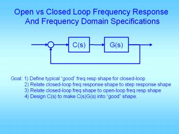
Open vs Closed Loop Frequency Response And
Frequency Domain Specifications
G(s)
C(s)
Goal 1) Define typical good freq resp shape
for closed-loop 2) Relate closed-loop
freq response shape to step response shape
3) Relate closed-loop freq shape to open-loop
freq resp shape 4) Design C(s) to make
C(s)G(s) into good shape.
2
(No Transcript)
3
Prototype 2nd order system closed-loop frequency
response
For small zeta, resonance freq is about wn BW
ranges from 0.5wn to 1.5 wn For good z range, BW
is 0.8 to 1.1 wn So take BW wn
z0.1
0.2
0.3
No resonance for z lt 0.7 Mr1dB for
z0.6 Mr3dB for z0.5 Mr7dB for z0.4
w/wn
4
0.2
z0.1
0.3
0.4
wgc
In the range of good zeta, wgc is about 0.65
times to 0.8 times wn
w/wn
5
In the range of good zeta, PM is about 100z
z0.1
0.2
0.3
0.4
w/wn
6
Important relationships
- Prototype wn, open-loop wgc, closed-loop BW are
all very close to each other - When there is visible resonance peak, it is
located near or just below wn, - This happens when z lt 0.6
- When z gt 0.7, no resonance
- z determines phase margin and Mp
- z 0.4 0.5 0.6 0.7
- PM 44 53 61 67 deg 100z
- Mp 25 16 10 5
7
Important relationships
- wgc determines wn and bandwidth
- As wgc ?, ts, td, tr, tp, etc ?
- Low frequency gain determines steady state
tracking - L.F. magnitude plot slope/(-20dB/dec) type
- L.F. asymptotic line evaluated at w 1 the
value gives Kp, Kv, or Ka, depending on type - High frequency gain determines noise immunity
8
Desired Bode plot shape
9
Proportional controller design
- Obtain open loop Bode plot
- Convert design specs into Bode plot req.
- Select KP based on requirements
- For improving ess KP Kp,v,a,des / Kp,v,a,act
- For fixing Mp select wgcd to be the freq at
which PM is sufficient, and KP 1/G(jwgcd) - For fixing speed from td, tr, tp, or ts
requirement, find out wn, let wgcd wn and
choose KP as above
10
(No Transcript)
11
(No Transcript)
12
- clear all
- n0 0 40 d1 2 0
- figure(1) clf margin(n,d)
- proportional control design
- figure(1) hold on grid Vaxis
- Mp 10/100
- zeta sqrt((log(Mp))2/(pi2(log(Mp))2))
- PMd zeta 100 3
- semilogx(V(12), PMd-180 PMd-180,'r')
- get desired w_gc
- xginput(1) w_gcd x(1)
- KP 1/abs(polyval(n,jw_gcd)/polyval(d,jw_gcd))
- figure(2) margin(KPn,d)
- figure(3) stepchar(KPn, dKPn)
13
(No Transcript)
14
(No Transcript)
15
n1 d1/5/50 1/51/50 1 0 figure(1) clf
margin(n,d) proportional control
design figure(1) hold on grid Vaxis Mp
10/100 zeta sqrt((log(Mp))2/(pi2(log(Mp))2)
) PMd zeta 100 3 semilogx(V(12),
PMd-180 PMd-180,'r') get desired
w_gc xginput(1) w_gcd x(1) Kp
1/abs(polyval(n,jw_gcd)/polyval(d,jw_gcd)) Kv
Kpn(1)/d(3) ess0.01 Kvd1/ess z w_gcd/5
p z/(Kvd/Kv) ngc conv(n, Kp1 z) dgc
conv(d, 1 p) figure(1) hold on
margin(ngc,dgc) ncl,dclfeedback(ngc,dgc,1,1)
figure(2) step(ncl,dcl) grid figure(3)
margin(ncl1.414,dcl) grid
16
(No Transcript)
17
(No Transcript)
18
(No Transcript)
19
(No Transcript)
20
(No Transcript)
21
(No Transcript)
22
(No Transcript)
23
KP/KD
20log(KP)
Place wgcd here
24
(No Transcript)
25
PD Control
- C(s)KP KDs KP(1TDs)
- For fixing wgcd and PMd
- Compute wgcd from tr, td, etc
- Compute PMd from Mp
- Compute f PMd PM_at_wgcd
- Compute TD tan(f)/wgcd
- KP 1/sqrt(1Td2wgcd2)/abs(G(jwgcd))
- KDKPTD
26
Example
C(s)
G(s)
Want maximum overshoot lt 10 rise
time lt 0.3 sec
27
(No Transcript)
28
(No Transcript)
29
- n0 0 1 d0.02 0.3 1 0
- figure(1) clf margin(n,d)
- Mp 10/100
- zeta sqrt((log(Mp))2/(pi2(log(Mp))2))
- PMd zeta 100 3
- tr 0.3 w_n1.8/tr w_gcd w_n
- PM angle(polyval(n,jw_gcd)/polyval(d,jw_gcd))
- phi PMdpi/180-PM Td tan(phi)/w_gcd
- KP 1/abs(polyval(n,jw_gcd)/polyval(d,jw_gcd))
- KP KP/sqrt(1Td2w_gcd2) KDKPTd
- ngc conv(n, KD KP)
- figure(2) margin(ngc,d)
- figure(3) stepchar(ngc, dngc)
Could be a little less
30
(No Transcript)
31
Less than spec
32
Variation
- Restricted to using KP 1
- Meet Mp requirement
- Find wgc and PM
- Find PMd
- Let f PMd PM (a few degrees)
- Compute TD tan(f)/wgcd
- KP 1 KDKPTD
33
(No Transcript)
34
(No Transcript)
35
- n0 0 5 d0.02 0.3 1 0
- figure(1) clf margin(n,d)
- Mp 10/100
- zeta sqrt((log(Mp))2/(pi2(log(Mp))2))
- PMd zeta 100 10
- GM,PM,wgc,wpcmargin(n,d)
- phi (PMd-PM)pi/180 Td tan(phi)/wgc
- KP1 KDKPTd
- ngc conv(n, KD KP)
- figure(2) margin(ngc,d)
- figure(3) stepchar(ngc, dngc)
36
(No Transcript)
37
(No Transcript)
38
- n0 0 5 d0.02 0.3 1 0
- figure(1) clf margin(n,d)
- Mp 10/100
- zeta sqrt((log(Mp))2/(pi2(log(Mp))2))
- PMd zeta 100 18
- GM,PM,wgc,wpcmargin(n,d)
- phi (PMd-PM)pi/180 Td tan(phi)/wgc
- Kp1 KdKpTd
- ngc conv(n, Kd Kp)
- figure(2) margin(ngc,d)
- figure(3) stepchar(ngc, dngc)
39
(No Transcript)
40
(No Transcript)
41
(No Transcript)
42
(No Transcript)
43
(No Transcript)
44
(No Transcript)
45
(No Transcript)


