Parabolic PDEs

1
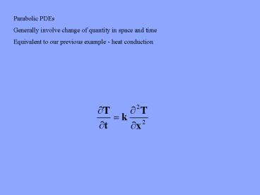
Parabolic PDEs Generally involve change of
quantity in space and time Equivalent to our
previous example - heat conduction
2
Can use the same grid idea, only boundaries are
different
time (j index)
space (i index)
3
Need initial conditions - green dots and boundary
conditions - red dots
One side of grid is always open
4

• Because parabolic PDEs are open-ended in time,
  can have instability
• Need to address this in solution methods
• Explicit
• Implicit

5
Explicit solutions Use finite differences
tj1
tj
xi
xi-1
xi1
6
Substitute into equation and rearrange
Explicit solution for this parabolic PDE
7
Example Given the initial condition and boundary
conditions below, solve for heat distribution
over time See matlab code
8
Stability conditions It can be shown that the
condition for stability is
or
look at what happens when you play with lambda
9

• Other points
• Can include derivative boundary conditions -
  introduce an imaginary point as in ellipitical
  example

Use finite difference for derivative to eliminate
imaginary point, introduce derivative into
propagation equation
10
We get
11
Can also use higher order temporal approximations
for time term (and for space term)
12

• Implicit methods
• avoid stability problems
• One example implicit method - use next time step
  to approximate spatial derivative

13
Substituting,
Three unknowns
14
Write these equations for all interior nodes -
you get enough equations Set up in matrix and get
a tridiagonal matrix Unconditionally stable -
although accuracy is degraded at larger ?t