The hazard function

1
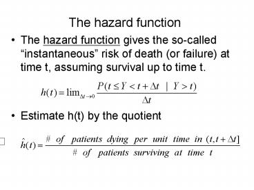
The hazard function

• The hazard function gives the so-called
  instantaneous risk of death (or failure) at
  time t, assuming survival up to time t.
• Estimate h(t) by the quotient

2

• The hazard function is also called the
  instantaneous failure rate or force of mortality
  or conditional mortality rate or age-specific
  failure rate. In a real sense it gives the risk
  of failure (death) per unit time over the
  progress of aging.
• We have seen f(y)-d/dy(S(y)),
• and so that f, S,
• and h are all related and each can be obtained
  from the others. Hazard functions can be flat,
  increasing, decreasing, or more complex

3
(No Transcript)
4

• Consider a simple hazard function, the constant
  hazard h(y)? for all y0. Here we assume ?????,
  where ???0. We have seen that
• so if we evaluate this for h(y) ?, we get
• Since f(y)-d/dy(S(y)), we have
• the exponential probability density with
  parameter ?. This means the expected value is ?
  and the variance is ?2.

5

• Definition 2.1 writes Y as Y exp(?? with
  h(y)1/? and notes that this is one of the most
  commonly used models for lifetime distributions.
  One reason is because of the memoryless
  property of the exponential distribution given
  on page 20
• Theorem 2.1 If Y exp(?? then for any ygt0 and
  tgt0 we have P(Ygtyt Ygty)P(Ygtt)
• Note this says that given survival past y, the
  conditional probability of surviving an
  additional t is the same as the unconditional
  probability of surviving t. Thus there is no
  aging with an increased risk of dying
• Go over Example 2.1 to see a picture of
  exponential data which would then have a constant
  hazard (of value 1/mean(Y))
• Note from Theorem 2.2 that if Y exp(?? , Y/?
  exp(1). This tells us that if we multiply an
  exponential survival variable by a constant, the
  MTTF is correspondingly multiplied by the same
  constant.

6

• How do we decided whether a set of survival data
  is following the exponential distribution? That
  the hazard is constant?
• Look over Example 2.1 - 200 randomly generated
  exponential variables with mean100.
  Characteristic skewed distribution, sample
  mean107.5, sample s.d.106.1 (Recall that if
  Yexp(?? then E(Y)SD(Y) ?. ) The sample
  stemplot and the sample mean and sd approximate
  the true shape, center and spread of the
  exponential.
• The estimated hazards (rightmost column) approx.
  .01 (1/100) - constant - see the formula on p.22
  for getting these values
• But another way to check the distribution is to
  compare the quantiles of the exponential
  distribution with the sample quantiles in a plot
  known as a qqplot. See R3 for a way to compute
  the quantiles and do the plot Recall that the
  p-th quantile of a distribution of a r.v. Y is
  the value Q s.t. P(YltQ)p. So we must compute
  the quantiles of the theoretical distribution and
  compare them (smallest to smallest, next smallest
  to next smallest, etc.) to the sample quantiles.

7

• Power Hazard
• Note this is of the form (constant)yconstant and
  if ??1 this reduces to the constant hazard we
  just considered.
• Note that and so
• We say in this case that Y Weibull(????. The
  mean and variance of Y are given in Theorem 2.5
  in terms of the gamma function
• Note that Y Weibull(1,???exp(???and if ?gt1 the
  hazard function is increasing if ??1, the hazard
  is decreasing if ??1 then the hazard is constant
  (as in the exponential survival case)
• Note that if ??2, the hazard is linear in y.
• Go over Example 2.2 on pages 24-25. Y
  Weibull(2,sqrt(3)). Use R (gamma()) to compute
  the values of the Gamma function Also in R,
  shapealpha and scalebeta in qweibull.

8

• To check graphically if a distribution is
  Weibull, do essentially a qqplot on the log-log
  scale (see section 4.4, p. 61-63). The key
  formulas are
• (4.2) Now substitute the ordered data and take
  natural logs
• (4.2a) Take logs again
• (4.2b)
• Write as a linear equation
• (4.3)
• (4.3a)
• So plot the points in 4.4, look for a straight
  line and the slope will equal 1/? and the
  intercept will equal log(?)