Simple Linear Regression - PowerPoint PPT Presentation
1 / 26
Title:
Simple Linear Regression
Description:
Simple Linear. Regression. Chapter 6. SHARON LAWNER WEINBERG. SARAH KNAPP ABRAMOWITZ ... When two variables are related, you may use one to predict the other. ... – PowerPoint PPT presentation
Number of Views:211
Avg rating:3.0/5.0
Title: Simple Linear Regression
1
Simple LinearRegression
SHARON LAWNER WEINBERG SARAH KNAPP ABRAMOWITZ
Statistics SPSS An Integrative
Approach SECOND EDITION
Using
- Chapter 6
2
Simple Linear Regression
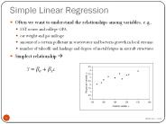
- When two variables are related, you may use one
to predict the other. The variable being
predicted is often called the dependent or
criterion or outcome variable. The variable
predicting the dependent variable is called the
independent variable, predictor or regressor. - In predicting one variable from another, we are
not suggesting that one variable is a cause of
the other.
3
Overview of Topics Covered
- Simple linear regression when both independent
and dependent variables are scale - The scatterplot Graphing the best-fitting
linear equation - The simple linear regression equation Yhat
bXa - The standardized regression equation
- R as a measure of the goodness of fit of the
model - Why the scatterplot is important
- Simple linear regression when the independent
variable is dichotomous
4
An Example Graphing the Simple Linear Regression
Equation on the Scatterplot for Predicting
Calories from Fat
- Go to Graphs on the Main Menu bar, Scatter, and
Define. Put CALORIES in the box for the Y-Axis
and FAT in the box for the X-Axis. Click OK. - Once the graph appears in the Output Navigator,
click it twice to go into Edit Mode. Go to
Elements on the menu bar, Fit Line at Total.
Click on Elements, Show Data Labels. - Note By convention, the dependent variable is on
the y-axis and the independent variable is on the
x-axis.
5
The Best-Fitting Line for Predicting Calories
from Fat
6
Using the Scatterplot to Predict the Number of
Calories of a Burger with 28 Grams of Fat
- Answer Approximately 520 calories.
- Note A Big Mac has 28 grams of fat, but actually
has 530 calories. The predicted value of 520
calories departs from the actual value by 10
calories. This amount, the difference, d,
between the actual and predicted values, is
called the residual or error. - In equation form, we may say that in this case,
- d Y 530 - 520 10
7
Creating the Best-Fitting Line Averaging (a
function of) the ds
- While d 10 in this case, d may equal a
different value for each of the other four cases
in this data set. - The line that best fits our data, in the sense
that it provides the most accurate predictions of
the DV, is the one that gives rise to the overall
smallest possible set of d values. - The overall set of d values is summarized as an
average, and, in particular, as an average of the
squared ds rather than as an average of the ds
themselves so as to avoid the cancelling out of
negative and positive ds when forming the
average. By squaring, we only are adding
positive terms to get the average.
8
Creating the Best-Fitting Line The Least Squares
Criterion
- Because we take an average of the squared ds to
find the best-fitting line, the criterion for
creating that line is called the Least Squares
Criterion. - The best-fitting line is called the (least
squares) regression line or (least squares)
prediction line. - The equation of the regression line is called the
linear regression equation.
9
The Regression Equation
- Although the derivation of the regression
equation is beyond the scope of this course, the
equation of the regression line itself is really
quite simple. - The regression line is given by
- where
10
Interpreting Regression Coefficients Slope, b
The value of the slope, b, gives the change in
the predicted value of Y, on average, for each
unit increase in X. If b is positive, then Y
increases with an increase in X . If b is
negative, then Y decreases with an increase in X.
11
Interpreting Regression Coefficients Intercept, a
The value of the intercept, a, is the predicted
value of Y when X 0. It is only meaningful
when 0 is a meaningful value for the variable X
and data close to X 0 have been
collected. Based on the equation for a, we may
note that a is defined so that when X , the
predicted value of Y is i.e. ( , )
lies on the regression line.
12
An Example Using SPSS to Obtain the Linear
Regression Equation for Predicting Calories from
Fat using the Hamburg Data Set
Go to Analyze on the Main Menu bar, Regression,
Linear. Put CALORIES in the box for the Dependent
variable and FAT in the box for the Independent
variable. To obtain the set of predicted Y
values and their residuals, click Save. In the
boxes labeled Predicted Values and Residuals,
click the boxes next to Unstandardized. Click
Continue, and OK. In the data window, you will
see that two new variables, PRE_1 and RES_1, have
been created which give predicted and residual
calories for each hamburger.
13
An Example Continued Writing the Regression
Equation
The regression equation may be obtained from the
output in the Coefficients table.
14
An Example Interpreting the Regression
Coefficients, b and a.
where Y Calories and X Fat
The value of the slope, b 13.71, tells us that
a one gram increase in the fat content of a
burger is associated with an increase of 13.71
calories, on average. The value of the
intercept, a 133.576, is not meaningful in this
example because burgers with 0 grams of fat would
be quite different from the burgers in this data
set.
15
An Example Continued Using the Regression
Equation to Predict Calories from a Burger with
28 Grams of Fat
Where Y Calories and X Fat
16
An Example Continued Reviewing the Data with
PRE_1 and RES_1
Burger Fat Calories Cheese PRE_1 RES_1
Hamburger 10 270 0 270.6751 -0.67513
Cheeseburger 14 320 1 325.5147 -5.51471
Quarter Pounder 21 430 0 421.484 8.51604
Quarter P. w/ c 30 530 1 544.873 -14.873
Big Mac 28 530 1 517.4532 12.54679
17
The Standardized Regression Equation
The regression equation for predicting the
standardized (z-score) values of Y from the
standardized (z-score) values of X is
18
Measuring the Goodness of Fit of the Model R
- R is defined as the correlation between the
actual and predicted values of Y. - In the case of simple linear regression
- As such, R may be used to measure how well the
regression model fits the data.
19
Drawing the Correct Conclusions Illustrating
with Anscombes Data
- Consider four data sets of X,Y pairs, each with
the following identical set of summary
statistics - 9.0, 7.5, SX 3.17, SY 1.94, rXY
.82 - Regression line 0.5X 3
- Question Can we draw the same conclusions about
each set of data? That is, are the four
scatterplots corresponding to these data sets the
same? Lets see.
20
Anscombes Data Panels I II
21
Anscombes Data Panel III IV
22
The Moral of the Story As Illustrated by
Anscombes Data
- Summary statistics, including the linear
regression model, may be misleading or in some
way fail to capture the salient features of data. - The use of graphical displays, such as the
scatterplot, is critical in the process of
assessing how appropriate a given model is for
describing a set of data.
23
Simple Linear Regression When the Independent
Variable is Dichotomous
- An Example Predict the number of calories in a
burger by whether or not the burger has cheese. - Find the regression equation using SPSS
- Predict the calories for a burger with cheese.
How else might we interpret this value? - Predict the calories for a burger without cheese.
How else might we interpret this value? - Find and interpret the intercept, a.
- Find and interpret the slope, b.
24
Simple Linear Regression When the Independent
Variable is Dichotomous
- The regression equation is
- Where X CHEESE and Y CALORIES
25
Simple Linear Regression When the Independent
Variable is Dichotomous
- The predicted calories for a burger with cheese
is (110)(1) 350 460. Intuitively, this is the
mean number of calories for burgers with cheese. - The predicted calories for a burger without
cheese is (110)(0) 350 350. Intuitively, this
is the mean number of calories for burgers
without cheese.
26
Simple Linear Regression When the Independent
Variable is Dichotomous
- The slope of the regression equation is 110,
indicating that burgers with cheese have 110 more
calories, on average, than burgers without
cheese. - The intercept of the regression equation is 350,
indicating that burgers without cheese are
predicted to have 350 calories. Note that in this
example, the value X0 is meaningful and
therefore, so is the intercept.


