Modelbased analysis, or datadriven modelling - PowerPoint PPT Presentation
1 / 18
Title:
Modelbased analysis, or datadriven modelling
Description:
in order to determine the state of the system. ... Alles folgende Material aus der Dissertation von Trygve Aspelien! Method (Nudging) ... – PowerPoint PPT presentation
Number of Views:31
Avg rating:3.0/5.0
Title: Modelbased analysis, or datadriven modelling
1
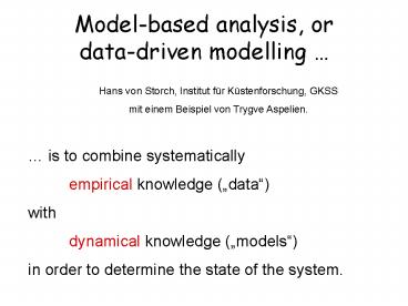
Model-based analysis, ordata-driven modelling
Hans von Storch, Institut für Küstenforschung,
GKSS mit einem Beispiel von Trygve Aspelien.
is to combine systematically empirical
knowledge (data) with dynamical knowledge
(models) in order to determine the state of the
system.
2
The knowledge represented by data and models are
both uncertain. This uncertainty makes us to
resort to statistical concepts. The resulting
additional knowledge is best guesses of the state
of the system (ideally together with confidence
intervals) This new knowledge claims are based
on the amount of available data. If more data are
available, the confidence in the numbers
increases.
3
- In general, the problem may be conceptualized by
the state space formalism, with - a state space
equation, e.g., - ?t1 F(?t, a, ?) e (M)
- with the state variable ?t, external parameters ?
and internal parameters a. The term e is a random
component, which supposedly represents the
uncertainty of the model M. - an observation equation
- xt B(?t) d (B)
- with the observable x, and the random component d.
4
Forward integration
Skillful estimates of the unknown field ?t are
obtained by integrating the state-space equations
and the observation equation forward in time
5
Beispiel Wasserstand in der Nordsee
- Dissertation von Trygve Aspelien, 2005 (GKSS)
- The use of long-term observations in combination
with modeling and their effect on the estimation
of the North Sea storm surge climate
Alles folgende Material aus der Dissertation von
Trygve Aspelien!
6
(No Transcript)
7
Method (Nudging)
Modeled sea level height ef is nudged towards the
measured sea eo for each gridpoint within an
area of influence
8
Reproduced variability
9
Sensitivity of the method
(a) Different choice of tide gauges (Aberdeen,
Whitby, Cromer)
Validation tide gauges
Normalized RMS
10
Whitby 60 km vs 30 km
Normalized RMS
11
Sensitivity of the method
All tide gauges, different decorrelation radii
(L), different nudging coefficients (a).
Validation tide gauges
Normalized RMS
12
Storm surge distribution (1958-2001)
- Control run is underestimating the surge
- Closer to the observed frequency distribution
after nudging - Especially for high and low surges
13
Spatial effects of nudging (1958-2001)
Average of differences (ABE-CTL) in the yearly
95th percentiles
Sea level height
Surge
14
Inter-annual variability (SLH) (1958-2001)
Annual mean high water (Cuxhaven)
- Positive bias in annual mean high water reduced
after nudging
- Long-term trend after nudging is closer to
observed trend
15
Inter-annual variability (surge) (1958-2001)
Cuxhaven
- After nudging
- Better reproduced inter-annual variability
Black curve observed values Blue curve Aberdeen
nudged (ABE) Red curve Control experiment (CTL)
- Linear long-term trends are closer to the
observed trends
- Improvement from CTL in the percentiles
(1,5,10,90,95,99) of surge when Aberdeen is
nudged (Brier skill score) - Cuxhaven 58-80
- Borkum 10-76
16
(No Transcript)
17
The Kalman filter
(Sequential method)
System Model Measurement Model
Initial Conditions Other Assumptions
State Estimate Extrapolation Error Covariance
Extrapolation
State Estimate Update Error Covariance
Update Kalman Gain Matrix
18
Experiments (II)
- (a) Different choice of tide gauges (Aberdeen,
Whitby, Cromer)
- (b) All available information
- (17 UK tide gauges)
- (c) Sensitivity of different decorrelation
radius (L)
- (d) Sensitivity of different nudging
coefficients (a)
(a)
(c)
(b)
(d)


