Point Estimation

1
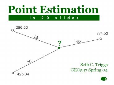
Point Estimation
i n 2 0 s l i d e s
286.50
774.52
25
?
20
30
Seth C. Triggs GEO597 Spring 04
425.34
2
What is point estimation?

• Point estimation is an estimation of a value
  based on the distance from the unknown. This is
  in a sense an application of Toblers First Law
  of Geography
• Close things are more related than far things!

3
Polygon usage

• Many triangulation methods involve polygons.

4
After figure 11.1
To create polygons of influence, draw
perpendicular bisectors! (also see figure 10.2 in
text)
EXAMPLE
5
Look at these sharp differences between the
polygons of influence! (after Figure 11.2)
6
Triangulation

• Politicians do it - many of us do it - it
  involves making a plane through three samples
  around the point of interest.
• This plane is a triangle and its slope represents
  the gradient between points.
• Equations

(11.2)
ax1 by1 c z1 ax2 by2 c z2 ax3 by3
c z3
(11.1)
z ax by c
7
(11.4)
(11.5)
(11.3)
Triangulation estimator v -11.25x 41.614y -
4421.159
63a 140b c 696 64a 129b c 227 71a
140b c 606
When solving, a -11.250, b 41.614, c
-4421.159
(65E, 137N) 548.7
Think of this like the slope of a mountain the
highest point is 696, then 606, then 227. You
could even map it and put contour lines on.
(after Figure 11.3)
8
Delaunay Triangulation

• This requires polygons of influence
• Three polygons must share a vertex.

(after figure 11.4)
9
Weighted Linear Combination

• Another type of triangulation estimate that
  produces a similar result.
• This one uses a single equation instead of three
  in regular triangulation.

(After Fig. 11.5)
J
(11.6)
AOIJ
AOJK
O
AOJK vI AOIK vJ AOIJ vK AIJK
vO
AOIK
K
I
10
Local Sample Mean

• By taking a local sample mean, we can get a
  quick and dirty method for estimation.

11
Inverse Distance Methods

• For each sample, the weight is inversely
  proportional to its distance from the point of
  interest.
• Thus, as distance decreases, weight increases.

(11.8)
n i1
1 di
vi
v
n i1
1 di
12
ID SAMP X Y V Dist 1/di (1/di)/(
1/di) 1 225 61 139 477 4.5 0.2222 0.2088 2 437 63
140 696 3.6 0.2778 0.2610 3 367 64 129 227 8.1 0.1
235 0.1160 4 52 68 128 646 9.5 0.1053 0.0989 5 259
71 140 606 6.7 0.1493 0.1402 6 436 73 141 791 8.9
0.1124 0.1056 7 366 75 128 783 13.5 0.0741 0.0696
1/di 1.0644
Mean is 603.7
After Table 11.2
13
Search Neighborhoods

• Sometimes we need to specify how far away we want
  to look to find a neighbor.
• You wouldnt want to hunt 500 miles for the
  nearest neighbor, because that could be expensive
  in terms of time.

14
Estimation Criteria

• These criteria differ by the distribution of your
  data. Youll get different results by changing p,
  the exponent.

(11.9)
1
n i1
vi
p i
d
v1
1
n i1
p i
d
15
For univariate estimate distributions

• You can compare the mean and standard deviation
  between the estimated and true values!

n
Mean Absolute Error (11.11)
1 n
r
i 1
MSE variance bias2
Mean Squared Error (11.12)
n
1 n
r2
i1
16
For univariate error distributions

• Youll want to have a small variance in
  residuals, not a small bias.
• There is a true value v and an estimated value v.
• Thus, the error is v - v r. Its also called a
  residual.

Based on figure 11.9
Less variance with bias
Large variance without bias
f
17
For bivariate estimated and true values

• If you plot your true versus predicted values,
  you can also get an indication of how well the
  model holds.
• The best values form a line of 45 degrees from
  the origin.

18
Some case studies

• Smoothing - sometimes estimated values have a
  smaller variance than sample values because
  estimations use weighted linear averages of
  several samples.
• Figure 11.13 gives an indication of the
  performance of the different estimation methods.
  Table 11.16 gives statistics.
• It appears that polygonal performs better.

(See figure 11.13)
19
Additionally

• We can look at how clustering affects samples and
  the estimates.
• Triangulation seems better because of its low
  standard deviation.
• Largest errors can be minimized by inverse
  distance weighing. See tables 11.7 and 11.8.

20
The End!

• An excellent antidote to PowerPoint poisoning is
  black coffee. Get it at your favorite coffee shop
  or convenience store.