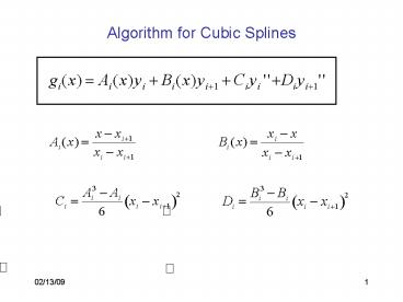
Algorithm for Cubic Splines

1
Algorithm for Cubic Splines
2
Boundary Condition for Natural Splines
Boundary conditions for a natural spline y0
yn 0
We can use the Thomas algorithm to solve the
tridiagonal systems of equations.
3
Difficult Data
4
Difficult Data
11 Points
Spline
The cubic spline interpolation does NOT
oscillates (at least not in this case)
5
Difficult Data
5 Points
6
Difficult Data
7 Points
7
Difficult Data
11 Points
8
Difficult Data
21 Points
9
A Constant Data Set
Use 11 constant support points
10
A Constant Data Set
Use 11 constant support points. Perturb the
middle one
The polynominal exhibits large oscillations away
from the perturbation.
11
A Straight Line with Small Random Noise
Use 21 constant support points. Small Random
Noise superposed.
12
The Cubic Spline Smoothness Theorem
If g(x) is the natural cubic spline function that
interpolates a twice-continuously differentiable
function f at knots a x0ltx1ltltxnb, then
13
The Cubic Spline Smoothness Theorem
If the last term on the rhs would be 0, we would
be finished because then
Lets use integration by parts to show that this
term is indeed 0
14
The Cubic Spline Smoothness Theorem
g is a cubic polynominal in each interval, ---gtgt
third derivative is a constant, ci, in each
interval.
15
Examples of Natural Cubic Spline Interpolation
16
Natural Cubic Spline Interpolation
17
1st and 2nd Derivatives from Cubic Splines
We can use cubic splines to obtain the first and
second derivative from a series of points
The 2nd derivative is a by-product of our
calculation of the cubic splines.
We had found before that the 1st derivative of a
cubic spline function is given by
18
The 1st Derivative
19
The 2nd Derivative
20
The Ionosphere over Logan
21
The Ionosphere over Logan
22
The Ionosphere over Logan
For many applications (for example ray tracing)
the 1st derivative of the density profile needs
to be known.