Inverse kinematics for our 2link robot' - PowerPoint PPT Presentation
1 / 80
Title:
Inverse kinematics for our 2link robot'
Description:
Note that there is a quadrant ambiguity for q2. Note that there is a quadrant ... for a digging task. ... Inverse kinematics for a digging task. Let point P ... – PowerPoint PPT presentation
Number of Views:144
Avg rating:3.0/5.0
Title: Inverse kinematics for our 2link robot'
1
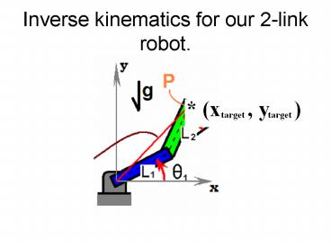
Inverse kinematics for our 2-link robot.
2
The goal is to place P on the target
3
The goal is to place P on the target
4
Let xtargetx, ytargety
5
(No Transcript)
6
(No Transcript)
7
Note that there is a quadrant ambiguity for q2.
8
Note that there is a quadrant ambiguity for q2.
9
(No Transcript)
10
Choice of sign determines elbow-up or elbow-down
option.
11
(No Transcript)
12
A two-argument function Resolves quadrant
ambiguity.
13
sin positive and cos positive.
14
sin positive and cos negative.
15
sin negative and cos positive.
16
sin negative and cos negative.
17
c12 c1c2-s1s2
18
(No Transcript)
19
(No Transcript)
20
(No Transcript)
21
(No Transcript)
22
(No Transcript)
23
(No Transcript)
24
Then
25
Then
26
Then
27
Then
28
Then
29
(No Transcript)
30
(No Transcript)
31
(No Transcript)
32
(No Transcript)
33
(No Transcript)
34
(No Transcript)
35
Inverse kinematics for a digging task.
36
We seek a kinematic solution for a portion of the
motion of a nonholonomic system
37
one that will duplicate the effect of the
following holonomic sequence.
38
one that will duplicate the effect of the
following holonomic sequence.
39
Inverse kinematics for a digging task.
40
Let point P track the target path.
41
Let point P track the target path.
42
Let point P track the target path.
43
At the same time, keep the knife edge aligned
with the tangent to the target path.
44
This is a three-degree-of-freedom task.
45
We seek, at each juncture along the length of the
trajectory to control 2 components of position of
point P ...
46
and one component of end-of-arm-tool
orientation.
47
We have three degrees of robot freedom in order
to realize these three objectives.
48
We have three degrees of robot freedom in order
to realize these three objectives.
49
We have three degrees of robot freedom in order
to realize these three objectives.
50
We have three degrees of robot freedom in order
to realize these three objectives.
51
We assume that the
Although q3 does entail rotation, it is not a
revolute joint in the sense that we have
considered such degrees of freedom in Craig.
52
We assume that the
Nevertheless in this limited context (of
simultaneous action of both wheels with no slip
on a flat surface) we could create a T(q1,q2,q3)
matrix to describe the forward kinematics of the
blue shovel
53
We assume that the
although it could not be made to fit the
Denavit Hartenberg convention, for example.
54
We assume that the
Rather than do that as the basis for our inverse
kinematics, we instead will work with a direct
model for the kinematics of P, as per HW1.
55
This is a planar task, and we assume that
previous action of the base has been conducted in
order to place the robot in the desired (near-)
vertical plane.
56
We will take x0, y0 to be the juncture at which
P would begin its action of traversing the red
dashed line.
57
We will take x0, y0 to be the juncture at which
P would begin its action of traversing the red
dashed line.
58
The coefficients Co C1 C2 of the path of the
line y(x)CoC1xC2x2 have been chosen in order
to produce a particular scoop volume.
59
Forward kinematics of OPX OPY and f.
60
f
61
q1
62
q2
63
f -q1 q2 - Y
64
f -q1 q2 - Y
65
OPY yp(q1,q2) L1 sin(q1) L2 sin(q1-q2)
y0
66
OPY yp(q1,q2) L1 sin(q1) L2 sin(q1-q2)
y0
67
OPX xp(q1,q2,q3) L1 cos(q1) L2
cos(q1-q2) Rq3 x0
68
OPX xp(q1,q2,q3) L1 cos(q1) L2
cos(q1-q2) Rq3 x0
69
OPX xp(q1,q2,q3) L1 cos(q1) L2
cos(q1-q2) Rq3 x0
70
OPX xp(q1,q2,q3) L1 cos(q1) L2
cos(q1-q2) Rq3 x0
x0 is known
71
x0 is known, together with y0
72
Also, L1 L2 and Y are known
x0 is known, together with y0
73
Note that, as things are defined, Co will always
be zero.
74
y(x)C1xC2x2
Note further that, as shown, C1 is negative, and
C2 positive.
75
y(x)C1xC2x2
Take xfinal to be the nonzero x such that
y(xfinal)0.
76
y(x)C1xC2x2
Take xfinal to be the nonzero x such that
y(xfinal)0, i.e. xfinal-C1/C2
77
y(x)C1xC2x2
Prob. 1a. For any x, 0ltxltxfinal, determine the
target angle f as defined herein. Be sure to
avoid quadrant ambiguities by using the
dual-argument inverse tangent of Craig. Generate
results in terms of C1 C2
78
y(x)C1xC2x2
Prob. 1b. For any x, 0ltxltxfinal, determine the
robot angles q1 q2 as defined herein. Do this in
radians and in terms of given yo L1 L2 Y C1 C2.
79
y(x)C1xC2x2
Prob. 1c. For any x, 0ltxltxfinal, determine the
robot angle q3 as defined herein. Do this in
radians and in terms of given xo yo L1 L2 Y C1 C2.
80
y(x)C1xC2x2
Prob. 1d. For all x, 0ltxltxfinal, given R150mm
L1300mm L2450mm Y1.0 radian C1-1 x018mm
y0150mm C2(500mm)-1, use your
inverse-kinematics relations of 1a-1c to make a
single plot superimposing each of the three robot
angles as functions of x.


![Forecast on China Industrial Robot Industry[2015-2019] PowerPoint PPT Presentation](https://s3.amazonaws.com/images.powershow.com/8334715.th0.jpg?_=20190501113)


