Outline

About This Presentation

Title:

Outline

Description:

... time clock period ... Clock cycle maximum computation time. Inefficient for average ... Non Atomic Data Value Reading. Receiver R1 gets (X=4, Y=5), R2 ... – PowerPoint PPT presentation

Number of Views:63

Avg rating:3.0/5.0

Slides: 95

Provided by: albertosan

Learn more at: https://ptolemy.berkeley.edu

Category:

more less

Transcript and Presenter's Notes

Title: Outline

1
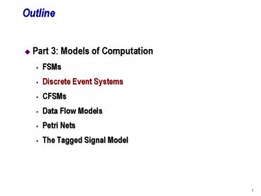
Outline

Part 3 Models of Computation
FSMs
Discrete Event Systems
CFSMs
Data Flow Models
Petri Nets
The Tagged Signal Model

2
Discrete Event

Explicit notion of time (global order)
Events can happen at any time asynchronously
As soon as an input appears at a block, it may be
executed
The execution may take non zero time, the output
is marked with a time that is the sum of the
arrival time plus the execution time
Time determines the order with which events are
processed
DE simulator maintains a global event queue
(Verilog and VHDL)
Drawbacks
global event queue gt tight coordination between
parts
Simultaneous events gt non-deterministic behavior
Some simulators use delta delay to prevent
non-determinacy

3
Simultaneous Events in DE
t
Fire B or C?
t
A
B
C
B has 0 delay
B has delta delay
t
t
t
t
A
B
C
A
B
C
Fire C once? or twice?
Fire C twice.

Can be refined
E.g. introduce timing constraints
(minimum reaction time 0.1 s)

Still have problem with 0-delay (causality) loop
4
Outline

Part 3 Models of Computation
FSMs
Discrete Event Systems
CFSMs
Data Flow Models
Petri Nets
The Tagged Signal Model

5
Co-Design Finite State MachinesCombining FSM
and Discrete Event

Synchrony and asynchrony
CFSM definitions
Signals networks
Timing behavior
Functional behavior
CFSM process networks
Example of CFSM behaviors
Equivalent classes

6
Codesign Finite State Machine

Underlying MOC of Polis and VCC
Combine aspects from several other MOCs
Preserve formality and efficiency in
implementation
Mix
synchronicity
zero and infinite time
asynchronicity
non-zero, finite, and bounded time
Embedded systems often contain both aspects

7
Synchrony Basic Operation

Synchrony is often implemented with clocks
At clock ticks
Module reads inputs, computes, and produce output
All synchronous events happen simultaneously
Zero-delay computations
Between clock ticks
Infinite amount of time passed

8
Synchrony Basic Operation (2)

Practical implementation of synchrony
Impossible to get zero or infinite delay
Require computation time ltltlt clock period
Computation time 0, w.r.t. reaction time of
environment
Feature of synchrony
Functional behavior independent of timing
Simplify verification
Cyclic dependencies may cause problem
Among (simultaneous) synchronous events

9
Synchrony Triggering and Ordering

All modules are triggered at each clock tick
Simultaneous signals
No a priori ordering
Ordering may be imposed by dependencies
Implemented with delta steps

10
Synchrony System Solution

System solution
Output reaction to a set of inputs
Well-designed system
Is completely specified and functional
Has an unique solution at each clock tick
Is equivalent to a single FSM
Allows efficient analysis and verification
Well-designed-ness
May need to be checked for each design (Esterel)
Cyclic dependency among simultaneous events

11
Synchrony Implementation Cost

Must verify synchronous assumption on final
design
May be expensive
Examples
Hardware
Clock cycle gt maximum computation time
Inefficient for average case
Software
Process must finish computation before
New input arrival
Another process needs to start computation

12
Pure Asynchrony Basic Operation

Events are never simultaneous
No two events have the same tag
Computation starts at a change of the input
Delays are arbitrary, but bounded

13
Asynchrony Triggering and Ordering

Each module is triggered to run at a change of
input
No a priori ordering among triggered modules
May be imposed by scheduling at implementation

14
Asynchrony System Solution

Solution strongly dependent on input timing
At implementation
Events may appear simultaneous
Difficult/expensive to maintain total ordering
Ordering at implementation decides behavior
Becomes DE, with the same pitfalls

15
Asynchrony Implementation Cost

Achieve low computation time (average)
Different parts of the system compute at
different rates
Analysis is difficult
Behavior depends on timing
Maybe be easier for designs that are insensitive
to
Internal delay
External timing

16
Asynchrony vs. Synchrony in System Design

They are different at least at
Event buffering
Timing of event read/write
Asynchrony
Explicit buffering of events for each module
Vary and unknown at start-time
Synchrony
One global copy of event
Same start time for all modules

17
Combining Synchrony and Asynchrony

Wants to combine
Flexibility of asynchrony
Verifiability of synchrony
Asynchrony
Globally, a timing independent style of thinking
Synchrony
Local portion of design are often tightly
synchronized
Globally asynchronous, locally synchronous
CFSM networks

18
CFSM Overview

CFSM is FSM extended with
Support for data handling
Asynchronous communication
CFSM has
FSM part
Inputs, outputs, states, transition and output
relation
Data computation part
External, instantaneous functions

19
CFSM Overview (2)

CFSM has
Locally synchronous behavior
CFSM executes based on snap-shot input assignment
Synchronous from its own perspective
Globally asynchronous behavior
CFSM executes in non-zero, finite amount of time
Asynchronous from system perspective
GALS model
Globally Scheduling mechanism
Locally CFSMs

20
Network of CFSMs Depth-1 Buffers

Globally Asynchronous, Locally Synchronous (GALS)
model

F
BgtC
CgtF
G
CgtG
CgtG
F(G1)
C
CgtA
CFSM2
CFSM2
CFSM1
CFSM1
C
CgtB
A
B
CgtB
(A0)gtB
CFSM3
21
Introducing a CFSM

A Finite State Machine
Input events, output events and state events
Initial values (for state events)
A transition function
Transitions may involve complex, memory-less,
instantaneous arithmetic and/or Boolean functions
All the state of the system is under form of
events
Need rules that define the CFSM behavior

22
CFSM Rules phases

Four-phase cycle
Idle
Detect input events
Execute one transition
Emit output events
Discrete time
Sufficiently accurate for synchronous systems
Feasible formal verification
Model semantics Timed Traces i.e. sequences of
events labeled by time of occurrence

23
CFSM Rules phases

Implicit unbounded delay between phases
Non-zero reaction time
(avoid inconsistencies when interconnected)
Causal model based on partial order
(global asynchronicity)
potential verification speed-up
Phases may not overlap
Transitions always clear input buffers
(local synchronicity)

24
Communication Primitives

Signals
Carry information in the form of events and/or
values
Event signals present/absence
Data signals arbitrary values
Event, data may be paired
Communicate between two CFSMs
1 input buffer / signal / receiver
Emitted by a sender CFSM
Consumed by a receiver CFSM by setting buffer to
0
Present if emitted but not consumed

25
Communication Primitives (2)

Input assignment
A set of values for the input signals of a CFSM
Captured input assignment
A set of input values read by a CFSM at a
particular time
Input stimulus
Input assignment with at least one event present

26
Signals and CFSM

CFSM
Initiates communication through events
Reacts only to input stimulus
except initial reaction
Writes data first, then emits associated event
Reads event first, then reads associated data

27
CFSM networks

Net
A set of connections on the same signal
Associated with single sender and multiple
receivers
An input buffer for each receiver on a net
Multi-cast communication
Network of CFSMs
A set of CFSMs, nets, and a scheduling mechanism
Can be implemented as
A set of CFSMs in SW (program/compiler/OS/uC)
A set of CFSMs in HW (HDL/gate/clocking)
Interface (polling/interrupt/memory-mapped)

28
Scheduling Mechanism

At the specification level
Should be as abstract as possible to allow
optimization
Not fixed in any way by CFSM MOC
May be implemented as
RTOS for single processor
Concurrent execution for HW
Set of RTOSs for multi-processor
Set of scheduling FSMs for HW

29
Timing Behavior

Scheduling Mechanism
Globally controls the interaction of CFSMs
Continually deciding which CFSMs can be executed
CFSM can be
Idle
Waiting for input events
Waiting to be executed by scheduler
Executing
Generate a single reaction
Reads its inputs, computes, writes outputs

30
Timing Behavior Mathematical Model

Transition Point
Point in time a CFSM starts executing
For each execution
Input signals are read and cleared
Partial order between input and output
Event is read before data
Data is written before event emission

31
Timing Behavior Transition Point

A transition point ti
Input may be read between ti and ti1
Event that is read may have occurred between ti-1
and ti1
Data that is read may have occurred between t0
and ti1
Outputs are written between ti and ti1
CFSM allow loose synchronization of event data
Less restrictive implementation
May lead to non intuitive behavior

32
Event/Data Separation

Value v1 is lost even though
It is sent with an event
Event may not be lost
Need atomicity

33
Atomicity

Group of actions considered as a single entity
May be costly to implement
Only atomicity requirement of CFSM
Input events are read atomically
Can be enforced in SW (bit vector) HW (buffer)
CFSM is guaranteed to see a snapshot of input
events
Non-atomicity of event and data
May lead to undesirable behavior
Atomicized as an implementation trade-off
decision

34
Non Atomic Data Value Reading

Receiver R1 gets (X4, Y5), R2 gets (X5 Y4)
X4 Y5 never occurs
Can be remedied if values are sent with events
still suffers from separation of data and event

35
Atomicity of Event Reading

R1 sees no events, R2 sees X, R3 sees X, Y
Each sees a snapshot of events in time
Different captured input assignment
Because of scheduling and delay

36
Functional Behavior

Transition and output relations
input, present_state, next_state, output
At each execution, a CFSM
Reads a captured input assignment
If there is a match in transition relation
consume inputs, transition to next_state, write
outputs
Otherwise
consume no inputs, no transition, no outputs

37
Functional Behavior (2)

Empty Transition
No matching transition is found
Trivial Transition
A transition that has no output and no state
changes
Effectively throw away inputs
Initial transition
Transition to the init (reset) state
No input event needed for this transition

38
CFSM and Process Networks

CFSM
An asynchronous extended FSM model
Communication via bounded non-blocking buffers
Versus CSP and CCS (rendezvous)
Versus SDL (unbounded queue variable topology)
Not continuous in Kahns sense
Different event ordering may change behavior
Versus dataflow (ordering insensitive)

39
CFSM Networks

Defined based on a global notion of time
Total order of events
Synchronous with relaxed timing
Global consistent state of signals is required
Input and output are in partial order

40
Buffer Overwrite

CFSM Network has
Finite Buffering
Non-blocking write
Events can be overwritten
if the sender is faster than receiver
To ensure no overwrite
Explicit handshaking mechanism
Scheduling

41
Example of CFSM Behaviors

A and B produce i1 and i2 at every i
C produce err or o at every i1,i2
Delay (i to o) for normal operation is nr, err
operation 2nr
Minimum input interval is ni
Intuitive correct behavior
No events are lost

42
Equivalent Classes of CFSM Behavior

Assume parallel execution (HW, 1 CFSM/processor)
Equivalent classes of behaviors are
Zero Delay
nr 0
Input buffer overwrite
ni?nr
Time critical operation
ni/2?nr?ni
Normal operation
nr?ni/2

43
Equivalent Classes of CFSM Behavior (2)

Zero delay nr 0
If C emits an error on some input
A, B can react instantaneously output
differently
May be logically inconsistent
Input buffers overwrite ni?nr
Execution delay of A, B is larger than arrival
interval
always loss of event
requirements not satisfied

44
Equivalent Classes of CFSM Behavior (3)

Time critical operation ni/2?nr?ni
Normal operation results in no loss of event
Error operation may cause lost input
Normal operation nr?ni/2
No events are lost
May be expensive to implement
If error is infrequent
Designer may accept also time critical operation
Can result in lower-cost implementation

45
Equivalent Classes of CFSM Behavior (4)

Implementation on a single processor
Loss of Event may be caused by
Timing constraints
nilt3nr
Incorrect scheduling
If empty transition also takes nr
ACBC round robin will miss event
ABC round robin will not

46
Some Possibility of Equivalent Classes

Given 2 arbitrary implementations, 1 input
stream
Dataflow equivalence
Output streams are the same ordering
Petri net equivalence
Output streams satisfy some partial order
Golden model equivalence
Output streams have the same ordering
Except reordering of concurrent events
One of the implementations is a reference
specification
Filtered equivalence
Output streams are the same after filtered by
observer

47
Conclusion

CFSM
Extension ACFSM Initially unbounded FIFO
buffers
Bounds on buffers are imposed by refinement to
yield ECFSM
Delay is also refined by implementation
Local synchrony
Relatively large atomic synchronous entities
Global asynchrony
Break synchrony, no compositional problem
Allow efficient mapping to heterogeneous
architectures

48
Outline

Part 3 Models of Computation
FSMs
Discrete Event Systems
CFSMs
Data Flow Models
Petri Nets
The Tagged Signal Model

49
Data-flow networks

A bit of history
Syntax and semantics
actors, tokens and firings
Scheduling of Static Data-flow
static scheduling
code generation
buffer sizing
Other Data-flow models
Boolean Data-flow
Dynamic Data-flow

50
Data-flow networks

Powerful formalism for data-dominated system
specification
Partially-ordered model (no over-specification)
Deterministic execution independent of scheduling
Used for
simulation
scheduling
memory allocation
code generation
for Digital Signal Processors (HW and SW)

51
A bit of history

Karp computation graphs (66) seminal work
Kahn process networks (58) formal model
Dennis Data-flow networks (75) programming
language for MIT DF machine
Several recent implementations
graphical
Ptolemy (UCB), Khoros (U. New Mexico), Grape (U.
Leuven)
SPW (Cadence), COSSAP (Synopsys)
textual
Silage (UCB, Mentor)
Lucid, Haskell

52
Data-flow network

A Data-flow network is a collection of functional
nodes which are connected and communicate over
unbounded FIFO queues
Nodes are commonly called actors
The bits of information that are communicated
over the queues are commonly called tokens

53
Intuitive semantics

(Often stateless) actors perform computation
Unbounded FIFOs perform communication via
sequences of tokens carrying values
integer, float, fixed point
matrix of integer, float, fixed point
image of pixels
State implemented as self-loop
Determinacy
unique output sequences given unique input
sequences
Sufficient condition blocking read
(process cannot test input queues for emptiness)

54
Intuitive semantics

At each time, one actor is fired
When firing, actors consume input tokens and
produce output tokens
Actors can be fired only if there are enough
tokens in the input queues

55
Intuitive semantics

Example FIR filter
single input sequence i(n)
single output sequence o(n)
o(n) c1 i(n) c2 i(n-1)

c2
i
c1

o
56
Intuitive semantics

Example FIR filter
single input sequence i(n)
single output sequence o(n)
o(n) c1 i(n) c2 i(n-1)

c2
i
c1

o
57
Intuitive semantics

Example FIR filter
single input sequence i(n)
single output sequence o(n)
o(n) c1 i(n) c2 i(n-1)

c2
i
c1

o
58
Intuitive semantics

Example FIR filter
single input sequence i(n)
single output sequence o(n)
o(n) c1 i(n) c2 i(n-1)

c2
i
c1

o
59
Intuitive semantics

Example FIR filter
single input sequence i(n)
single output sequence o(n)
o(n) c1 i(n) c2 i(n-1)

c2
i
c1

o
60
Intuitive semantics

Example FIR filter
single input sequence i(n)
single output sequence o(n)
o(n) c1 i(n) c2 i(n-1)

c2
i
c1

o
61
Intuitive semantics

Example FIR filter
single input sequence i(n)
single output sequence o(n)
o(n) c1 i(n) c2 i(n-1)

c2
i
c1

o
62
Intuitive semantics

Example FIR filter
single input sequence i(n)
single output sequence o(n)
o(n) c1 i(n) c2 i(n-1)

c2
i
c1

o
63
Intuitive semantics

Example FIR filter
single input sequence i(n)
single output sequence o(n)
o(n) c1 i(n) c2 i(n-1)

c2
i
c1

o
64
Intuitive semantics

Example FIR filter
single input sequence i(n)
single output sequence o(n)
o(n) c1 i(n) c2 i(n-1)

c2
i
c1

o
65
Questions

Does the order in which actors are fired affect
the final result?
Does it affect the operation of the network in
any way?
Go to Radio Shack and ask for an unbounded queue!!

66
Formal semantics sequences

Actors operate from a sequence of input tokens to
a sequence of output tokens
Let tokens be noted by x1, x2, x3, etc
A sequence of tokens is defined as
X x1, x2, x3,
Over the execution of the network, each queue
will grow a particular sequence of tokens
In general, we consider the actors mathematically
as functions from sequences to sequences (not
from tokens to tokens)

67
Ordering of sequences

Let X1 and X2 be two sequences of tokens.
We say that X1 is less than X2 if and only if (by
definition) X1 is an initial segment of X2
Homework prove that the relation so defined is a
partial order (reflexive, antisymmetric and
transitive)
This is also called the prefix order
Example x1, x2 lt x1, x2, x3
Example x1, x2 and x1, x3, x4 are
incomparable

68
Chains of sequences

Consider the set S of all finite and infinite
sequences of tokens
This set is partially ordered by the prefix order
A subset C of S is called a chain iff all pairs
of elements of C are comparable
If C is a chain, then it must be a linear order
inside S (otherwise, why call it chain?)
Example x1 , x1, x2 , x1, x2, x3 ,
is a chain
Example x1 , x1, x2 , x1, x3 , is
not a chain

69
(Least) Upper Bound

Given a subset Y of S, an upper bound of Y is an
element z of S such that z is larger than all
elements of Y
Consider now the set Z (subset of S) of all the
upper bounds of Y
If Z has a least element u, then u is called the
least upper bound (lub) of Y
The least upper bound, if it exists, is unique
Note u might not be in Y (if it is, then it is
the largest value of Y)

70
Complete Partial Order

Every chain in S has a least upper bound
Because of this property, S is called a Complete
Partial Order
Notation if C is a chain, we indicate the least
upper bound of C by lub( C )
Note the least upper bound may be thought of as
the limit of the the chain

71
Processes

Process function from a p-tuple of sequences to
a q-tuple of sequences
F Sp -gt Sq
Tuples have the induced point-wise order
Y ( y1, , yp ), Y ( y1, , yp ) in Sp
Y lt Y iff yi lt yi for all 1 lt i lt p
Given a chain C in Sp, F( C ) may or may not be a
chain in Sq
We are interested in conditions that make that
true

72
Continuity and Monotonicity

Continuity F is continuous iff (by definition)
for all chains C, lub( F( C ) ) exists and
F( lub( C ) lub( F( C ) )
Similar to continuity in analysis using limits
Monotonicity F is monotonic iff (by definition)
for all pairs X, X X lt X gt F( X ) lt F(
X )
Continuity implies monotonicity
intuitively, outputs cannot be withdrawn once
they have been produced
timeless causality. F transforms chains into
chains

73
Least Fixed Point semantics

Let X be the set of all sequences
A network is a mapping F from the sequences to
the sequences
X F( X, I )
The behavior of the network is defined as the
unique least fixed point of the equation
If F is continuous then the least fixed point
exists LFP LUB( Fn( , I ) n gt 0 )

74
From Kahn networks to Data Flow networks

Each process becomes an actor set of pairs of
firing rule
(number of required tokens on inputs)
function
(including number of consumed and produced
tokens)
Formally shown to be equivalent, but actors with
firing are more intuitive
Mutually exclusive firing rules imply
monotonicity
Generally simplified to blocking read

75
Examples of Data Flow actors

SDF Synchronous (or, better, Static) Data Flow
fixed input and output tokens
BDF Boolean Data Flow
control token determines consumed and produced
tokens

1

1
1
T
F
select
merge
F
T
76
Static scheduling of DF

Key property of DF networks output sequences do
not depend on time of firing of actors
SDF networks can be statically scheduled at
compile-time
execute an actor when it is known to be fireable
no overhead due to sequencing of concurrency
static buffer sizing
Different schedules yield different
code size
buffer size
pipeline utilization

77
Static scheduling of SDF

Based only on process graph (ignores
functionality)
Network state number of tokens in FIFOs
Objective find schedule that is valid, i.e.
admissible
(only fires actors when fireable)
periodic
(brings network back to initial state firing
each actor at least once)
Optimize cost function over admissible schedules

78
Balance equations

Number of produced tokens must equal number of
consumed tokens on every edge
Repetitions (or firing) vector vS of schedule S
number of firings of each actor in S
vS(A) np vS(B) nc
must be satisfied for each edge

np
nc
A
B
79
Balance equations

Balance for each edge
3 vS(A) - vS(B) 0
vS(B) - vS(C) 0
2 vS(A) - vS(C) 0
2 vS(A) - vS(C) 0

80
Balance equations

M vS 0
iff S is periodic
Full rank (as in this case)
no non-zero solution
no periodic schedule
(too many tokens accumulate on A-gtB or B-gtC)

81
Balance equations

Non-full rank
infinite solutions exist (linear space of
dimension 1)
Any multiple of q 1 2 2T satisfies the
balance equations
ABCBC and ABBCC are minimal valid schedules
ABABBCBCCC is non-minimal valid schedule

82
Static SDF scheduling

Main SDF scheduling theorem (Lee 86)
A connected SDF graph with n actors has a
periodic schedule iff its topology matrix M has
rank n-1
If M has rank n-1 then there exists a unique
smallest integer solution q to
M q 0
Rank must be at least n-1 because we need at
least n-1 edges (connected-ness), providing each
a linearly independent row
Admissibility is not guaranteed, and depends on
initial tokens on cycles

83
Admissibility of schedules

No admissible schedule
BACBA, then deadlock
Adding one token (delay) on A-gtC makes
BACBACBA valid
Making a periodic schedule admissible is always
possible, but changes specification...

84
Admissibility of schedules

Adding initial token changes FIR order

i
i(-1)
i(-2)
c2
c1

o
85
From repetition vector to schedule

Repeatedly schedule fireable actors up to number
of times in repetition vector
q 1 2 2T
Can find either ABCBC or ABBCC
If deadlock before original state, no valid
schedule exists (Lee 86)

86
From schedule to implementation

Static scheduling used for
behavioral simulation of DF (extremely efficient)
code generation for DSP
HW synthesis (Cathedral by IMEC, Lager by UCB, )
Issues in code generation
execution speed (pipelining, vectorization)
code size minimization
data memory size minimization (allocation to
FIFOs)
processor or functional unit allocation

87
Compilation optimization

Assumption code stitching
(chaining custom code for each actor)
More efficient than C compiler for DSP
Comparable to hand-coding in some cases
Explicit parallelism, no artificial control
dependencies
Main problem memory and processor/FU allocation
depends on scheduling, and vice-versa

88
Code size minimization