Forecasting For Operational Decisions

1
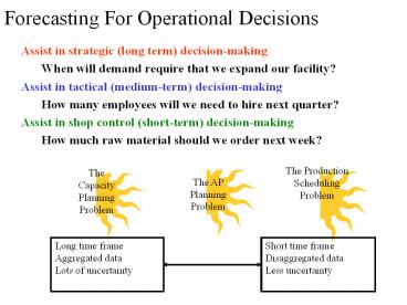
Forecasting For Operational Decisions

• Assist in strategic (long term) decision-making
• When will demand require that we expand our
  facility?
• Assist in tactical (medium-term) decision-making
• How many employees will we need to hire next
  quarter?
• Assist in shop control (short-term)
  decision-making
• How much raw material should we order next week?

Long time frame Aggregated data Lots of
uncertainty
Short time frame Disaggregated data Less
uncertainty
2
Forecasting Methods
Time frame of decision
short
long
much
Quantitative tools that can incorporate current
information. - Averaging - Exponential smoothing
Quantitative tools that can incorporate a great
deal of historical information. - Causal
methods - Time series
Experience with decision
Qualitative tools that use very rich sources of
data. - Judgement methods - Market research
none
3
(No Transcript)
4

• Goals
• Predict future from past
• Smooth out noise
• Standardize forecasting procedure

5
Patterns in Time-Series Data
TREND
Sale of fuel oil in gallons
CYCLE
SEASON
RANDOM
Time
6
Time Series Forecasting
Forecast
Historical Data
Time series model
A(i), i 1, ,t
f(tt), i 1, 2,
7
Moving Average

• Average most current values to predict future
  outcomes. The trend-cycle can be estimated by
  smoothing the series to reduce random variation.
• Assumptions
• No trend
• Equal weight to last m observations
• Model

8
Averaging Techniques Example
What if we used a three period moving average but
weighted the historical data as follows nearest
periods weight .6, second periods weight .3
and most distant period .1? What are the
advantages and disadvantages of using a weighted
average?
9
(No Transcript)
10
(No Transcript)
11
(No Transcript)
12
(No Transcript)
13
Cum error cum ave abs error
Running MAD
-19.54 Cumulative Forecast Error 151.58 Mean
Squared Error 12.31 Standard Deviation
8.81 Mean Absolute Deviation -.0729 Mean
Percent Error 0.1742 Mean Abs. Percent Error
14
Exponential Smoothing

• Estimate next outcome with a weighted combination
  of the forecast for previous period and the most
  recent outcome
• Assumptions
• No trend
• Exponentially declining weight given to past
  observations
• Model

F(t) Forecast in period t x(t) Actual demand
in period t smoothing constant is alpha
15
.1(20.2).9(10.5) 11.47
.65(27.60).35(41.48) 32.46
16
Exponential Smoothing with a Trend

• Assumptions
• Linear trend
• Exponentially declining weights to past
  observations/trends
• Model

F(t) Forecast in period t x(t) Actual demand
in period t ? ? smoothing constants (values
between 0 and 1) T(t) Trend component in period
t
17
Example Single Exponential Smoothing with
Trend Use last problems data to provide a SEST
forecast (?.55 ? .09)
Period 3 From period 2 x(2) 20.2, F(2)
10.5, T(2) 0
16.31
Period 4 From period 3 x(3) 23.9, F(3)
15.83, T(3) .48
21.34
Period 5 ?
18
Double Exponential Smoothing

• Special case of the Holts linear method - where
  the two parameters (? ?) assumed to be equal.
• Model

F(t) Forecast in period t x(t) Actual demand
in period t ? smoothing constant
19
Double Exponential Smoothing Use last problems
data to provide a DES forecast (?.79)
Period 3 From period 2 x(2) 20.2, F(2)
10.5
Period 4 From period 3 x(3) 23.9, F(3)
18.16, F(3)16.55
Period 5 ?
20
(No Transcript)
21
(No Transcript)
22
(No Transcript)
23
(No Transcript)
24
Regression of original and deseasonalized data
253.05 2.5615 291.4 (291.4).93 271.0
Reseasonalized (intercepttrend)season
25
Regression Equation for Deseasonalized data
253.05 2.56P
26
(No Transcript)
27
Forecasting example You must prepare a forecast
of product demand in order to plan for
appropriate production quantities. You receive
the following historical information from
marketing Month Sales
Advertising in thousands
in thousand s 1 264 2.5 2 116 1.3 3 165
1.4 4 101 1.0 5 209 2.0
28
(No Transcript)
29
(No Transcript)
30
Conclusions

• Sensitivity Lower values of m or higher values
  of a will make moving average and exponential
  smoothing models (without trend) more sensitive
  to data changes (and hence less stable).
• Trends Models without a trend will underestimate
  observations in time series with an increasing
  trend and overestimate observations in time
  series with a decreasing trend.
• Smoothing Constants Choosing smoothing constants
  is an art the best we can do is choose constants
  that fit past data reasonably well.
• Seasonality Methods exist for fitting time
  series with seasonal behavior (e.g., Winters
  method), but require more past data to fit than
  the simple models given here.
• Judgement No time series model can anticipate
  structural changes not signaled by past
  observations these require judicious overriding
  of the model by the user.