PACS CQMAVM ILT

1
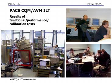
PACS CQM/AVM ILT
Results of functional/performance/ calibration
tests
2
Major (science) requirements on PACS
Spectroscopy
Photometry
Detectors Sensitivity Detector/readout noise
(NEP) Dynamic Range Chopper Stray Light Image
Quality
Few x 10-18 W/m2 (5s, 1hr) 5 x 10-18 W/Hz1/2

Few mJy (5s, 1hr) 1 x 10-16 W/Hz1/2
- 10000 Jy
- 3000 Jy
3
Major (science) requirements on PACS
Detectors Sensitivity, Detector/readout noise
(NEP), Dynamic Range Image Quality blur,
distortion, misalignment Spectral resolution,
wavelength range, filter bands, photometric
accuracy, .... Chopper frequency, duty cycle,
stability on plateau, position accuracy, range
(throw) Calibration Sources time constants,
stability, emissivity Stray Light homogeneous,
inhomogeneous
See PACS Science Requirement Document PACS
Instrument Requirement Document More PACS
Sub-unit specifications and requirements
documents...
4
(No Transcript)
5

• Two cryogenic test phases (19-23 July, 6 Sep-29
  Oct)
• Functional and Performance tests of all
  mechanisms, detectors, array read-outs, sensors
  and sources (?Test/Analysis Reports), including
  Test Optics
• Calibration tests (? calibration files, reports)
• S/W tests and improvements (QLA, TA, IA, e.g.
  visualization, detector sorting, de-compression)
• Tests/debugging of warm electronics (e.g.
  DEC/MEC)
• Tests of command scripts (Tcl, CUS), On-Board
  Control Procedures (OBCPs), Astronomical
  Observation Templates (AOT)

6
(No Transcript)
7
(No Transcript)
8
I) S/W and Warm Electronics
9
Detector Sorting Bolometer (IA Display Tool)

• Bolc Simulator Test Pattern
• reconstructed
• Figure by IA Display tool

Bolometer Blue
Bolometer Red
10
Detector Sorting Spectrometer
11
Detector Sorting Spectrometer
(Status GeGa arrays pixel performance (SCOS
result))
12
Detector Sorting Spectrometer
(Status GeGa arrays pixel performance (SCOS
result))
13
PACS - QLA
14
IA Plot / Display

• Setting saving Plot settings
• Labels, Axis, zooming, hardcopy,
• plotsymbols, ...
• Plot to PS without rendering
• Well documented

15
II) Functional/Performance tests and instrument
characterisation
16
(No Transcript)
17
(No Transcript)
18
(No Transcript)
19
Cross-reference major (science) requirements on
PACS vs. PCD
Detectors Sensitivity 3.2.1, 3.2.6,
4.3.8 Detector/readout noise (NEP) 1.1.11,
1.1.12, 1.2.10 Dynamic range 1.2.3,
4.3.6 Image Quality blur, distortion,
misalignment, PSF, ... 3.1.2, 3.1.3, 3.1.4,
4.1.1, 4.1.2, 4.1.3 Spectral resolution
4.2.2 Chopper frequency, duty cycle,
stability on plateau, position accuracy, range
(throw) 0.7.5, 0.7.6, 0.7.13, 2.3.2 Calibration
Sources time constants, stability, emissivity
0.7.11, 0.7.12 Stray Light, ghosts 3.1.5,
3.1.6, 4.2.4
20
II A) Photometer functional tests and
characterisation
21
Performed tests (photometer)
- 0.7.1 FPU thermal behaviour (photometer) -
0.7.2 Test of cooler recycling and operation -
0.7.4 Verify function of bolometer detectors -
0.7.5/6 and 2.3.2 Verify function of PACS
chopper / performance test / duty cycle - 0.7.7
Verify function of photometer filter wheels -
0.7.11/12 Verify function of internal
calibration sources / performance test - 1.1.1
Control optimum pixel bias setting - 1.1.10
Measure time constants after a flux change -
1.1.11 Measure the low frequency noise - 1.1.12
Measure the bolometer Noise Equivalent Power (NEP)
22

• - 2.2.3 Optimum positioning of chopper on
  internal reference sources (bolometer)
• - 2.5.1 Temporal stability of internal
  calibration sources
• - 2.5.3/0.7.12 Time constants heat-up
  cool-down times of internal calibration sources
• 3.1.1 Central pointing position (photometer)
• 3.1.2 Relation between chopper position and
  angular displacement on sky
• 3.1.4 Photometer Point Spread Function (PSF)
• 5.1.1 OBCP and AOT tests
• many ad hoc tests (including tests of test
  equipment/test optics)
• Conclusion Tests were often hampered by DECMEC
  problems. Bolometer sufficiently tested for
  CQM ILT purposes

23
Example 1 - Chopper FT, duty cycle

• Analysis of the waveform of the chopper
  modulation for different chopping frequencies and
  chopper deflections both for rectangular
  (two-position) and triangular (three-position)
  chopping.
• Duty cycle requirements
• On sky gt80 for 0-10 Hz chopping
  frequency
• On Cal. Sources gt 70 (larger throw)

24
Commanded vs. actual (read-back) chopper position
against time
25
Actual chopper position vs. Time (here 0.8 Hz,
1.2 degrees)
Fluctuations well within spec
26
Mean duty cycle for different chopping
frequencies vs. chopping throw
Here square modulation
27
Comparison to measure- ments of Zeiss Compared to
CQM measure- ments shorter swinging-in phase with
smaller amplitude. Plateaux much smoother.
Requirements fulfilled for all frequencies and
deflections. ? poorly adjusted DEC/MEC control
parameters ?
28
Example 2 PACS Calibration Sources
Analysis of the time constants and stability of
the two internal calibration sources.
29
Heat-up and temperature plateau behaviour (after
DECMEC adjustments)
30
Emissivity of calibration sources measured
against OGSE cryogenic blackbody. Values close to
design value.
31
Emissivity of calibration sources measured
against OGSE cryogenic blackbody. Values close to
design value.
32
Example 3 Bolometer flat field and offset
Discarded pixels
Module 5
Module 1
Module 2
Image of the offset
Image of the flat-field (gain)
pchopper position Ttemperature
s(i, j, p, T) o(i, j) g(i, j) f(i, j, p, T)
measured signal
input signal
33
Example 4 Photometer Field of View Chopper
Step-Scan Across PACS FOV

• Astronomical field cold OGSE BB
• Internal calibrators set to 70 K (left) and 90 K
  (right)
• No flatfielding applied

34
Example 4 - Chopper Step-Scan Across PACS FOV
35
Chopper position
36
Example 5 - First Point Source Image (Blue
Photometer)

• Point source hole with equiv. diam. 7 (2
  pixels) in front of external blackbody
• Blue photometer, on-array chopping nodding to
  remove very uneven OGSE background, no flat-field

• Point source hole with equiv. diam. 7 (2
  pixels) in front of external blackbody, on-array
  choppingnodding

• Point source hole with equiv. diam. 7 (2
  pixels) in front of external blackbody, on-array
  choppingnodding
• Same source, line scanning mode, unprocessed
  data

beam
- beam
37

• PSF wider than expected (25-50). This
  discrepancy clealy needs investigation. Part
  (most?) of it may be due to the imperfect focus
  of the PACS/OGSE setup and to the non-nominal
  plate scale.
• Strehl ratio can not be determined reliably right
  now.

Sigma of a 2D gaussian fit to the PSF of measured
and simulated data
38

• Summary of preliminary analysis
• OGSE external focus off the design position
• PSF wider than expected (25-50)
• Misalignments (1-4 degrees) between XY stage,
  chopper, arrays and subarrays
• Plate scale of the OGSE/PACS setup (mm on XY
  stage vs. pixels on detector array) is 10 off
  the design value. Assumed explanation caused by
  de-focus.
• Several of these results imply modifications of
  OGSE setup, test procedure and/or planning of FM
  tests. But there are no implications for CQM IST
  at this point.

39
Example 6 Time constants after switch-on
OGSE BB1 (29K) and 2 (6.5K), OGSE chopper wheel
at 500mHz
40
Example 6 Time constants after switch-on

• Bolometer signal roughly stabilized within 2
  hours after the switch-on
• Implications for observing strategy will be
  discussed at AOT workshop

41
Example 7 Bolometer Responsivity, Noise
Spectrum, NEP
Responsivityon OGSE BBs 1 x 1010 V/W
NEP 5 x 10-16 W/Hz1/2,as measured at
subunitlevel tests
42
Example 7 Bolometer Responsivity, Noise
Spectrum, NEP
43
II B) Spectrometer functional tests and
characterisation
44
Performed tests (spectrometer)
- 0.7.1 FPU thermal behaviour (spectrometer) -
0.7.3 Verify function of GeGa detectors, CREs,
detector heaters and related temperature
sensors many CRE tests for testing of
compression/de-compression, DECMEC etc. - 0.7.5/6
Verify function of PACS chopper (spectrometer),
performance test - 0.7.7 Verify function of
spectrometer filter wheels - 0.7.8 Verify
function of grating - 0.7.11/12 Verify function
of internal calibration sources / performance
test - 1.2.1 Optimum detector bias settings -
1.2.3 Dynamic range per selected integration
capacitor - 1.2.4 CRE check-out voltage -
1.2.6 Detector dark current - 1.2.11 Linearity
of CRE readout - 2.3.2 Duty cycle of chopper
waveforms
45
- 2.3.3 Optimum positioning of chopper on
internal reference sources (spectrometer) - 2.5.2
Spatial stability of internal calibration
sources - 4.1.1 Spectrometer central pointing
position and grating alignment - 4.1.3
Spectrometer PSF - 4.2.1 Grating wavelength
calibration - 4.3.2 Flux reproducibility
internal sources - 4.3.4 Flux reproducibility
external sources - 4.3.5 Linearity with flux -
4.3.8 Relative Spectral Response Function
spectrometer - 5.2.1/2 OBCP tests, calibration
AOT - Spectral map focal plane - Attempts with
external laser - many ad hoc tests (in particular
to debug DECMEC, CRE tests) ? Conclusion Tests
were often hampered by DECMEC problems (including
CRE settings) and by spectrometer filter wheel
being stuck.
46
Example 8 grating drive performance
Oscillations within specs
47
Example 9 grating wavelength calibration
Against water vapor absorption spectrum, Input
source external BB, 25.4mm, T730C, absorption
path in air 20 cm
48
Example 9 grating wavelength calibration
49
Example 9 grating wavelength calibration
The S/N on quite a number of pixels and a number
of lines has been very poor, such that
substructure in the continuum may cause apparent
shifts of the measured peak positions. Strongly
fringed pixels in the red section have not been
used in this analysis. The accuracy of the
reference water spectrum is limited, air
temperature and pressure have not been monitored
and no other air species than H2O have been
included in the calculations. Some small
systematic offsets for blended water lines may
therefore be present in the reference list. Given
these problems, no attempt has been made to
improve further on the calibration accuracy, by
fitting correction polynomials to individual
modules/pixels. The present accuracy for the red
spectrometer is of the order of a resolution
element while for the blue section it is better,
more of the order half to a third of a spectral
resolution element.
50
Example 10 Fringes
51
Example 11 Spectral resolution and Instrumental
Profile
52
Example 12 Spectral Leakage and Ghosts
2nd order leaking into 1st order (dichroic
cut-off), plus 0th order ?
3rd order leaking into 2nd order (blue filter
cut-off)
Strong narrow features beyond band limit (?)
53
Example 12 Spectral Leakage and Ghosts
Multiple reflections of 2nd order leaking into
1st order (?)
Angular dependent filter transmission (?)
54
Example 7 grating scans/stray light
55
Example 13 grating health checks/change in
behaviour
Hall sensors vs. Grating position over time
Spectrum vs. Grating position over time
(This occured after DECMEC malfunction had driven
grating against hard stop at full speed)
56
Example 9 - First (Water) Spectra (Spectrometer)

• Look out of the cryostat window toward Hg arc
  lamp through lab air
• Internal blackbody for reference

57
Example 14 - First Point Source Image
(Spectrometer)

• Point source hole with equiv. diam. 7 (1
  pixel) in front of external blackbody
• Blue spectrometer, (source on) (source
  off)(averaged over the 16 spectral channels of
  each spatial pixel)

Good agreementwith predicted PSF
58
Example 15 Linearity of CRE read-out
Analysis of the linearity of the integration
ramps of the illuminated detector pixels of the
red and blue spectrometer array. The required
accuracy is less than 3 deviation from a first
order fit The chopper position for all files was
at -24700 ADcounts (-10 degrees) which is outside
the science and even calibration window.
Consequently, the detectors detected not the OGSE
black body radiation but only stray
light! Measurements still usefull (e.g.
linearity, stability of ramp slope, etc.), but no
trend with temperature measurable.
59
Example 15 Linearity of CRE read-out
8Hz oscillations
Open channel subtracted
The non-linearities decrease significantly, the
hook in the beginning of the ramp is almost gone
and the oscillation behaviour is strongly
reduced. This indicates that a correlated
disturbing signal is modulated on the ramps of
all pixels of a module.
60
Example 15 Linearity of CRE read-out
- Different commanded OGSE black body temperature
values do not affect the slopes of the ramps.
This seems to be caused by a chopper position
outside the measuring windows at which the
detectors only see stray light. - The ramps
exhibit a starting hook and superimposed
oscillations mainly at a frequency of 8 Hz and
harmonics. The subtraction of the open channel
output decreases these effects substantially and
leads to a ramp almost perfectly linear. - The
responsivity variations of the pixels within a
module slightly exceed the requirement
specifications of 30. (Could be inhomogenous
illumination, though) - The stability of the
output signal shows a range of 8 to 35 and is
consequently far beyond the requirement
specification of 1. - The current noise density
is around 8 10-15 AHz-1/2 and exceeds the
requirement specification of 7 10-17 AHz-1/2 by
a factor of about 100 (but unsure due to the
unknown voltage range corresponding to the ADC
range). - The non-linearity of the ramps is about
10. Consequently, the requirement specification
of 3 is not fulfilled. This high non-linearity
is mainly caused by the first max. 13 ramp
read-outs (starting hook). This analysis should
be repeated using ramps with a higher dynamic
range and a better number statistics.
61
Example 16 Signal/Noise Measurements (Red
Module, QM5)
S/N ratio as measured during module tests
re-established during ILT with full signal/data
chain
Measurement in detector test cryostat (MPE
electronics)
Measurement in PACS (DECMEC)
62
Example 16 Signal/Noise Measurements (Blue
Module)
(FM42)
Measurement in detector test cryostat (MPE
electronics)
Measurement in PACS (DECMEC)
63
Example 17 Dark Current
64
Example 17 Dark Current
Dark current determination (preliminary!) Dark
current of Idark,195 4.3 10-14 A or 270000
e-/s. This would be a factor of 5.4 above the
specs. The signals refer, however, to the CFOV
measurement, which might not be completely dark,
so that the derived value must be considered as
an upper limit.
Comparison with results from module level tests
(preliminary!) Dark current measurements of
unstressed detector arrays carried out at MPIA
yielded dark currents between 1 and 3 10-13 A
for the temperature range 1.7 to 2.9K. The
derived dark current for pixel ID 195 (which is a
high stressed pixel) is a factor of 2.3 smaller
than the lowest values found for the blue
(unstressed) detector modules on module level.
65
Example 17 Optimum Detector Bias
The purpose of these calibration test (1.2.1 and
1.2.2) is to find the optimum bias voltage and
temperature range where the detector operates
under stable conditions and the NEP shows a
minimum. During CQM tests the heater on the blue
detector array housing was not functional,
therefore the detectors were kept at FPU
temperature without active regulation. The
optimisation procedure under these circumstances
was restricted to a bias scan at constant FPU
temperature. In this DRAFT version no NEP was
calculated but s(si/median(s)) was derived
instead, where si represents the the individual
slopes on subramps and median(s) is the
absolute value of slopes median. This measure is
proportional to the NEP, the derived minima will
not change when switching to NEP.
66
Example 17 Optimum Detector Bias
blue
red
The mean value in the red is 75 mV.
The mean value in the blue is 200 mV.
Preliminary!
67
III) OBCPs, AOT definition
68

• At present the following Observing modes are
  offered by PACS
• Line Spectroscopy
• Range Spectroscopy
• Dual band photometry
• Single band photometry
• (basically as fall back or for parallel mode
  with SPIRE)
• They will be commanded via On-Board Command
  Procedures (OBCPs), e.g.
• OBCP8 Grating Line scan with 2 or 3 position
  chopping
• OBCP5 Photometry with 2 or 3 position chopping
  with dither
• OBCP 10 Internal calibration I

69

• Each AOT consists in principle of
• AOT specific setup
• OBCP
• Change_Setup
• OBCP
• Change_Setup
• OBCP
• ...
• ...
• Change_Setup
• OBCP
• AOT specific reset

70

• One example for an AOT (chopped photometry) was
  already implemented as CUS script (incl. OBSID
  and BBID).
• OBCPs (the AOT building blocks) and dedicated
  AOT tests were performed in ILT.
• A (2-day) workshop is planned (17-18 January
  2005) to discuss further strategies for the
  (intimately linked) issues of AOT design,
  calibration files, and data analysis
• Next Milestones
• End 2004 Proof of concept
• Mid 2005 Deliver parameter sets/AOT definitions
  and observing time calculator - -
• End 2005 update calibration files (e.g.
  sensitivities) for time calculator

71

• One example for an AOT (chopped photometry) was
  already implemented as CUS script (incl. OBSID
  and BBID).
• OBCPs (the AOT building blocks) and dedicated
  AOT tests were performed in ILT.
• Map making strategies (e.g. scanning vs.
  rastering) are currently analyzed at NHSC, using
  the PACS Observation Simulator (performance
  problems need to be overcome)
• A (2 day) workshop is planned (17-18 January
  2005) to discuss further strategies for the
  (intimately linked) issues of AOT design,
  calibration files, and data analysis
• Next Milestones
• End 2004 Deliver observing time calculator
  for all PACS AOTs

72
HSPOT communicates with the CUS Engine. All
parameters are passed from HSPOT to the CUS
Engine. Any calculations are done in the CUS
Engine, because all logic is contained in the CUS
script.
PACS will not provide a stand-alone time
calculator but a first version of the AOT logic.
The AOT logic is implemented in CUS scripts. AOT
execution times will be calculated there. In
addition to the time calculator the CUS engine
will also contain a noise estimator (based for
now on theoretical expectations).
73
Cross-reference major (science) requirements on
PACS vs. PCD
Detectors Sensitivity 3.2.1, 3.2.6,
4.3.8 Detector/readout noise (NEP) 1.1.11,
1.1.12, 1.2.10 Dynamic range 1.2.3,
4.3.6 Image Quality blur, distortion,
misalignment, PSF, ... 3.1.2, 3.1.3, 3.1.4,
4.1.1, 4.1.2, 4.1.3 Spectral resolution
4.2.2 Chopper frequency, duty cycle,
stability on plateau, position accuracy, range
(throw) 0.7.5, 0.7.6, 0.7.13, 2.3.2 Calibration
Sources time constants, stability, emissivity
0.7.11, 0.7.12 Stray Light, ghosts 3.1.5,
3.1.6, 4.2.4
74
III) EMC Tests
75
Example 19 RS - H Field, Red and Blue Bolometers