Part 2 Stock Challenge

1
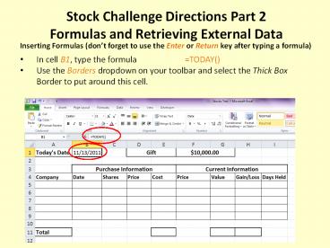
Stock Challenge Directions Part 2 Formulas and
Retrieving External Data
Inserting Formulas (dont forget to use the Enter
or Return key after typing a formula)

• In cell B1, type the formula TODAY()
• Use the Borders dropdown on your toolbar and
  select the Thick Box Border to put around this
  cell.

2

• In the cell H1, type the formula F1-E11
• Use the Borders dropdown on your toolbar and
  select the Thick Box Border to put around this
  cell.
• Format the cell by using Control1, Number tab,
  and select Currency.
• The Decimal places should read 2, Symbol should
  be a , and choose the red selection without
  parentheses for Negative numbers.

3

• In cell E5, type the formula C5D5
• Use the smart copy and paste feature to put
  this formula in E6 through E9

4

• In cell G5, put the formula F5C5
• Use smart copy and paste to put this formula in
  G6 through G9

5

• In cell H5, put the formula G5-E5
• Use smart copy and paste to put this formula in
  H6 through H9

6

• In cell E11, put the formula SUM(E5E9)
• (This can also be done by selecting E11, the
  Sigma key on the toolbar and then selecting E5
  through E9)

7

• In cell G11, put the formula SUM(G5G9)

8

• In cell H11, put the formula G11-E11

9

• In cell I5, put the formula B1-B5
• After entering this formula autosize the column.
• To make the absolute value read correctly, click
  the comma symbol on the toolbar under the Home
  Tab in the Number section.

10

• Click the Decrease Decimal icon on the toolbar in
  the same section to get rid of decimals if they
  appear. Dont worry if you get an odd number
  this will fix itself after one day on its own.

11
Use smart copy and paste to put this formula in
I6 through I9 (dont worry if the cell gives you
a strange answer with that formula ... it will
eventually fix itself as we go further in the
directions and time passes) .
12

• Conditional Formatting to add stationary
  background color to rows.
• Select cells B3-I3. Then, hold down the control
  key and also select A4 through I9.
• Select the Conditional Formatting dropdown
• Select New Rule
• Select Use a formula to determine which cells to
  format.
• In Format values where this formula is true put
  the formula
• MOD(ROW(),2)
• Choose the background fill color by selecting
  Format then from the Fill tab, select a light
  shade pastel color.

13

• Follow the same process again select the same
  cells, and conditional format with a second
  formula
• AND(MOD(ROW(),2)0)
• Shade this formula with an opposing light shade
  pastel color You will end up with something like
  the picture below.

14

• Select cells A11, E11, G11, and H11 (remember,
  using the control key lets you select
  non-contiguous cells).
• Use the paintbucket icon on the toolbar to choose
  a contrasting light pastel fill color that is
  different from the other 2 previously chosen.