ECCO Achievements, Capabilities, Applications, and Future Plan

1
ECCO Achievements, Capabilities, Applications,
and Future Plan
Tony Lee, NASA JPL/Caltech
http//www.ecco-group.org
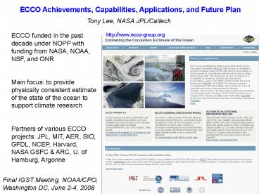
ECCO funded in the past decade under NOPP with
funding from NASA, NOAA, NSF, and ONR Main
focus to provide physically consistent estimate
of the state of the ocean to support climate
research Partners of various ECCO projects JPL,
MIT, AER, SIO, GFDL, NCEP, Harvard, NASA GSFC
ARC, U. of Hamburg, Argonne
Final IGST Meeting, NOAA/CPO, Washington DC, June
2-4, 2008
2
ECCO Capabilities and Achievements

• Inverse estimation of the time-varying state of
  the global ocean (along with the estimation of
  initial boundary conditions parameters).
• Product serving a suite of products (from
  multi-decadal to eddy-permitting) served through
  LAS, DODS, OPeNDAP.
• The physical consistency of ECCO products (e.g.,
  consistent estimate of state and forcing and
  state, budget closure) is crucial to climate
  diagnostics.
• Budget components of T S part of ECCO products.
• Adjoint tool for sensitivity analysis (process
  study Obs. Sys. evaluation).
• Online tracer tools to study water-mass pathways
  (origin and destination) using forward adjoint
  of passive-tracer equations based on ECCO-JPL
  product.
• Development of an open-source automatic
  differentiation tool.

3
ECCO-GODAE MIT adjoint-based estimation

• Assimilate a large suite of existing in-situ
  satellite data using the adjoint method by
  adjusting prior surface forcing initial
  conditions.
• MITOGCM, 1x1, 23 levels
• Delayed mode (1 year lag)
• Current product period 1992-2006

G-ECCO similar system, also a large ste. of data
constraints, product 1950-2000
4
ECCO-GODAE JPL Kalman filter/smoother assimilation
http//ecco.jpl.nasa.gov/

• Assimilate altimeter-derived SSH in-situ T
  profiles using Kalman filter/smoother method.
• MITOGCM MOM4, 1x0.3 in tropics, 1x1
  extra-tropics, 46 levels.
• Near real time (10-30 days lag).
• Product period 1993 onward.

5
ECCO-2 High-res. Global-Ocean Sea-Ice Data
Synthesis
http//ecco2.org

• MITOGCM (Cubed-sphere)
• 18x18 km, 50 levels
• Product 1992-2006
• Greens function method
• Data constraint
• - SSH mean anomaly
• - T S profiles (XBT, CTD, ARGO, TAO)
• - SST (GHRSST)
• - Sea ice concentration (SSMI)
• - Sea ice motion (radiometers, QuikSCAT, RGPS)
• - Sea ice thickness (ULS)

Control parameters Initial T S atmospheric
surface boundary conditions background vertical
diffusivity critical Richardson numbers for KPP
air-ocean, ice-ocean, air-ice drag coefficients
ice/ocean/snow albedo coefficients bottom drag
and vertical viscosity
6
Product Validation Examples
Described in various publications for different
subject of investigations
Comparison of mixed-layer temperature near cold
tongue between ECCO-JPL product (curve) and TAO
data (dots) (Kim et al. 2007)
Comparison of mixed-layer temperature velocity
in tropical Indian Ocean between ECCO-JPL product
RAMA mooring data (Halkides Lee 2008)
7
Evaluation of newly released ECCO-2
high-resolution Product using TAO mooring data at
a tough location
ECCO-2 release 1
TAO
ECCO-2 baseline
8
Evaluation of newly released ECCO-2
high-resolution Product using TAO mooring data
0N, 165E
0N, 110W
9
Applications of ECCO products tools for research

• A wide-range of topics including (not limited
  to)
• Data assimilation model improvement
• Ocean circulation
• Mixed-layer heat budget
• Sea level variability and changes
• Initialization of S-I prediction
• Biogeochemistry
• Geodesy
• Providing open-boundary conditions for regional
  systems.
• Over 150 peer-reviewed publications in the past
  decade (not including many external-user
  publications)

10
Application example
Mixed-layer temperature (MLT) balance in
southeastern tropical Indian Ocean (SETIO)
(Halkides Lee 2008)
The eastern box defined by Saji et al. (1999)
spans areas with different forcing ocean
dynamics. Differences in processes controlling
MLT within the box need to be understood.
Variance of horizontal advective tendency suggest
potential effects of equatorial currents in Box
1, coastal currents in Box 2, and South
Equatorial Current in Box 3.
11
Application example
MLT budget in SETIO for 1994, 1997, 2006 IODZM
events spatially inhomogenous event dependent
(Halkides Lee 2008)
Box 1 equatorial
Horizontal advection warms in Box 1 but cools in
Boxes 2 3 during IOZDM cooling
Box 2 coastal
Subsurface processes cools in Boxes 1 2 but
warms in Box 3 during IOZDM cooling
Box 3 SEC
Horiz. Advection in Box 1 help terminate cooling
in 94 06 but not 97
Made possible by budget closure
12
CO2
Application example
Importance of physical consistency to
interdisciplinary applications (McKinley 2002)
CO2 flux in tropical Pacific during ENSO inferred
from a Kalman filter estimation (physically
inconsistent) is unrealistically large (left),
but that based on Kalman filter-smoother
(physically consistent) is reasonable (right).
Kalman Filtered estimate
Kalman-filter/smoother estimate
13
Application example
Variability of N. Atl. Meridional Overturning
Circulation (Wunsch and Heimbach 2007)
Vertical distribution of volume transport (upper)
mid-depth transport time series (lower)

• No significant slowdown of Atlantic MOC found.
• Serious issue of potential aliasing for analysis
  based on infrequent hydrographic sections because
  of large month-to-month synoptic fluctuations.

14
Application example
Understanding decadal sea-level patterns (Wunsch
et al. 2007)
??T

• Vertical partition in density trends due to
• trends in temperature T
• trends in salinity S
• trends in T, S

??TS
??S
15
DJF hindcast for March initial conditions
Application example
Improvement of seasonal climate forecast by using
ECCO-JPL product as initial state in a coupled
model (UCLA atmos. Coupled to MITOGCM)
ECCO
baseline
persistence
Anomaly correlation increases with ECCO
ECCO
baseline
Cazes-Boezio, Menemenlis, and Mechoso, 2008 J.
Climate, 21, 1929-1947 .
persistence
Standard error reduces with ECCO
16
Future Plan of ECCO

• Sustain production and accelerate improvement in
  support of climate research (e.g., CLIVAR
  sciences).
• Sustaining production of delayed-mode
  adjoint-based estimation system.
• Near real-time extension using Kalman
  filter/smoother.
• Enhancement of resolution.
• Improvement of error covariance.
• Expansion of control space (e.g., including
  mixing coeff.)
• Longer term coupling with atmosphere
  biogeochemistry.