Introduction to Finite Element Methods

1
Introduction to Finite Element Methods
ME6443, Dr. A.A. Ferri
x
u1
u2
2
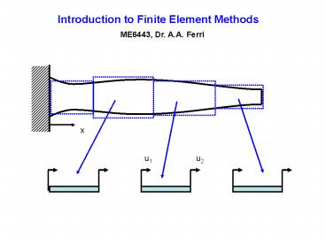
Within each element, we have a particular E, A, L
u1
u2
x
Assume a linear displacement field (exact for
statics.) Need to relate the 2 generalized
coordinates for each element to the displacement
field within each element. Assume a linear
displacement field
1
1
The functions N(x) are termed shape functions and
they are just Ritz functions that are local to
each element.
3
Element potential energy
We can also consider a distributed force per unit
length on each element
u1
u2
f(x)
P1
P2
x
Elemental virtual work can be expressed as
Lets take P1 P2 zero for now it will be
easy to put them back later.
4
Variational Principle
Assuming that the duis are independent and
arbitrary, we get
i 1,2
5
What if there are 2 elements?
element 1
element 2
E1, A1, L1
E2, A2, L2
0

combine
0
6
Thus, the global or unassembled static
equations are
But the global coordinate vector
has 1 too many degrees of freedom if the elements
are connected.
The coordinates of uG and U U1 U2 U3 T
are related as follows
4x3 compatibility matrix
7
Substitue S into global relationship
Now, premultiply by ST to eliminate equations
and preserve symmetry
Any nodes that are fixed have zero displacement.
Therefore, we can just delete the rows and
columns of K and the rows of F corresponding
to any fixed nodes
Nodal forces
If a force P is applied to node 1 of element n,
then the additional contribution to the elemental
force vector is P 0 T likewise, if the force
P is applied to node 2 of element n, then the
additional contribution to the elemental force
vector is 0 P T
8
Axial Deformation of a Tapered Rod
Example
A(x)A0(2-x/L)
P
Le
x
Consider N elements, each having length Le L/N
and area Ai
(midpoints)
where
9
Steel beam, of length 1 meter, and end width
20mm, and end thickness 4mm E2e11
rho7800 L1 A00.020.004 P 10000
N 1
ke 1.0e007 2.4000 -2.4000
-2.4000 2.4000
10
N 2
compatibity matrix
S 1 0 0 0 1 0 0
1 0 0 0 1
K 96000000 -40000000 -40000000
40000000
F 0 10000
Reduced
11
N 5
12
N 7
cond(K) 84.6059
K 1.0e008 4.1600 -2.0000 0
0 0 0 0
-2.0000 3.8400 -1.8400 0 0
0 0 0 -1.8400 3.5200
-1.6800 0 0 0 0
0 -1.6800 3.2000 -1.5200 0
0 0 0 0
-1.5200 2.8800 -1.3600 0 0
0 0 0 -1.3600 2.5600
-1.2000 0 0 0 0
0 -1.2000 1.2000
Note that, for N 7, K is 7x7 and symmetric.
It is also banded. We say that the bandwidth
of the matrix is 3. This diagonal dominance
of the stiffness matrices from finite-element
procedures is one of the reasons that the
condition number stays reasonable, even for
models having a large number of elements.
13
Connection to Global Ritz-Function Approach
6
5
3
4
1
2
x/Le
Using the admissible Ritz functions above would
yields identical results to those produced using
N 7 finite-elements (provided that areas
were staircased according to the same scheme
used with the FEM.